Implementation of Deep Neural NetworkAfter knowing the process of Backpropagation lets start and see how a deep neural network is implemented using PyTorch. The process of implementing a deep neural network is similar to the implementation of the perceptron model. There are the following steps which we have to perform during the implementation. Step 1: In the first step, we will import all the require libraries such as a torch, numpy, datasets, and matplotlib.pyplot. Step 2: In the second step, we define no of data points, and then we create a dataset by using make_blobs() function, which will create a cluster of the data point. Step 3: Now, we will create our dataset, and we will store our data points into the variable x while storing values into the variable y and we will make use of our label just a bit. Step 4: Now, we change make_blobs () to make_cicrcle() because we want dataset in a circular form. We pass appropriate argument in make_circle() function. The first argument represents the no of sample points, the second argument is random state, and the third argument is noise which will refer to the standard deviation of the Gaussian noise, and the fourth arguments are the factor which will refer to the relative size of the smaller inner circular region in comparison to the larger. Step 4: Now, after customizing our dataset as desired, we can plot it and visualize it using plt.scatter() function. We define x and y coordinates of each label dataset. Let's begin with the dataset which label is 0. It plots the top region of our data. Scatter function for 0 labeled dataset is defined as 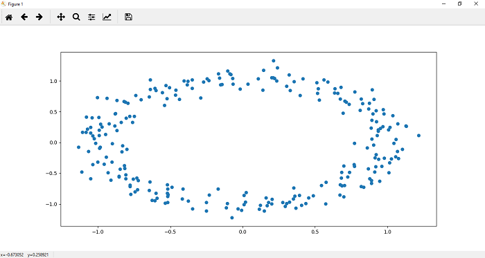 Step 5: Now, we plot the points in the lower region of our data. The scatter function () for one labeled dataset is defined as 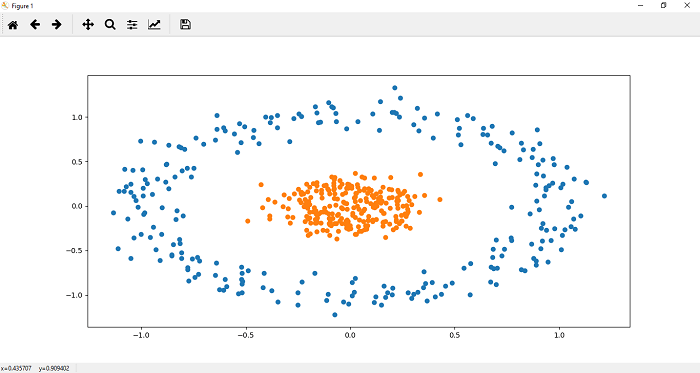 A single line can not classify the above dataset. For classifying this dataset will require a much deeper neural network. We put plt.scatter(x[y==0,0],x[y==0,1]) and plt.scatter(x[y==1,0],x[y==1,1]) into a function for further use as Step 6: In this step, we will create our model class as we have implemented in linear regression and perceptron model. The difference is that here we use the hidden layer also in between the input and output layer. In init() method, we will pass an addition argument h1 as a hidden layer, and our input layer is connected with the hidden layer, and the hidden layer is then connected with the output layer. So Now, we have to add this extra hidden layer in our forward function So that any input must be passed through the entire depth of the neural network for prediction to be made. So Our initialization is finished, and now, we are ready to use it. Keep in mind to train a model x, and y coordinates both should be numpy array. So what we do we will change our x and y values into tensor like Step 7 We will initialize a new linear model using Deep_neural_network() constructor and pass input_size, output_size and hidden_size as an argument. We now, print the random weight and biased values which were assigned to it as follows: Before this, to ensure consistency in our random result, we can seed our random number generator with torch manual seed, and we can put a seed of two as follow Step 8: The criterion by which we will compute the error of our model is recalled Cross entropy. Our loss function will be measured based on binary cross entropy loss (BCELoss) because we are dealing with only two classes. It is imported from an nn module. Now, our next step is to update parameters using the optimizer. So we define the optimizer which is used gradient descent algorithm. Here, we will use Adam optimizer. Adam optimizer is one of the many optimization algorithms. The Adam optimization algorithm is a combination of two other extensions of stochastic gradient descent such as Adagrad and RMSprop. Learning rate plays an important role in optimization. If we choose a minimal learning rate, it leads to very slow convergence towards the minimum and if you choose very large learning rate can hinder the convergence. The Adam optimizer algorithm ultimately computes the adaptive learning rate for each parameter. Step 9: Now, we will train our model for a specified no of epochs as we have done in linear model and perceptron model. So the code will be similar to perceptron model as 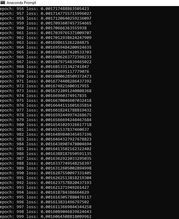 |
We provides tutorials and interview questions of all technology like java tutorial, android, java frameworks
G-13, 2nd Floor, Sec-3, Noida, UP, 201301, India


