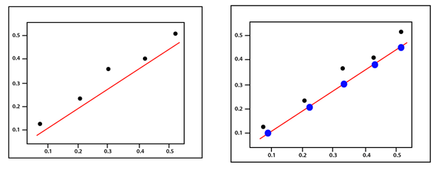
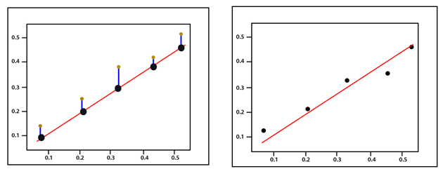
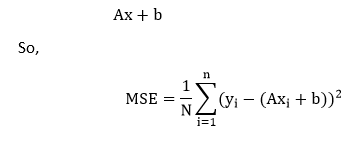
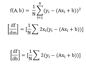
Mean Squared Error

Mean Squared Error is calculated in much the same way as the general loss equation from earlier. We will consider the bias value as well since that is also a parameter that needs to be updated during the training process.

(y-Ax+b)²

The mean squared error is best explained with an illustration.

Suppose we have a set of values and we start by drawing some regression line parameter sized by a random set of weight and bias value as before.

The error corresponds to how far the actual value is from the predicted value - the actual distance between them.

For each point, the error is calculated by comparing the predicted values which are made by our line model with the actual value using the following formula

Every point is associated with an error, which means we have to do the summation of the error for each point. We know the prediction can be rewritten as

As we are calculating the mean squared error, we have to take the average by dividing by the no of data points. Now mentioned before the gradient of the error function should take us in the direction of the greatest increase in error.

Moving towards the negative of the gradient of our cost function, we move in the direction of the smallest error. We will use this gradient as a compass to always take us in downhill. In gradient descent, we ignore the presence of bias, but for the error, both parameters A and b are required to define.

Now, what we do next we will calculate the partially derivatives for each and as before we start with any A and b value pair.

We use a gradient descent algorithm to update A and b in the direction of least error based on two partial derivatives which are mentioned above. For every single iteration, the new weight is equal to the

A₁=A₀-∝ f'(A)

And the new bias value is equal to

b₁=b₀-∝ f'(b)

The main idea for writing the code, i.e., we start with some random model with a random set of weight and bias value parameters. This random model will tend to have a large error function, a large cost function, and we then use gradient descent to update the weight of our model in the direction of the least error. Minimizing that error to return an optimized result.