| |

How to Use RIGHT Function in ExcelRight Function in ExcelThe RIGHT Function is part of the Excel TEXT functions category. The RIGHT function will return a specified number of characters from the end of a given text string. It aids in the extraction of characters from the rightmost to the left side. The result depends on the number of characters specified in the formula. For example, "=RIGHT("JAVATPOINT",5)" gives "POINT" as a result. The RIGHT function is helpful if we want to extract characters from the right side of a text string. Usually, it is used by combining it with other functions such as VALUE, COUNT, DAY, DATE, SUM, etc. SyntaxThe RIGHT function's syntax is as follows:
RIGHT(text, [num_chars])
Arguments
Characteristics of the Num_Chars"The following are the characteristics of the num_chars:
Note
How to Use RIGHT Function in Excel?We mostly used the RIGHT function in combination with other Excel functions such as FIND, SEARCH, LEFT, LEN, etc. The following are the uses of the RIGHT function:
Let us understand the use of the RIGHT function with the help of the following example: Example 1: In this example, there is a test string in cell A3, as we can see in the below screenshot. We need to extract the last word having 10 letters. 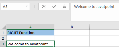
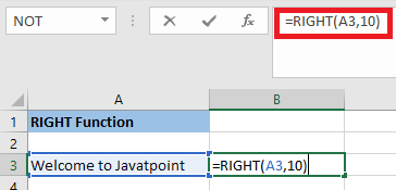
We will apply the RIGHT function in order to extract "string" in A3 column. We will use the below formula: =RIGHT(A3,10)
After applying the formula, the result would be: 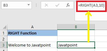
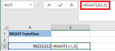
Example 2: In this example, we have an 8-digit number (98231212), and we have to extract the last 5 digits from this number. 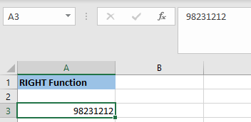
In order to extract the last 5 digits, we have to apply the following formula: =RIGHT(A3,5)
The RIGHT function returns 31212, as we can see in the below screenshot: 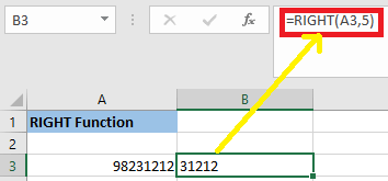
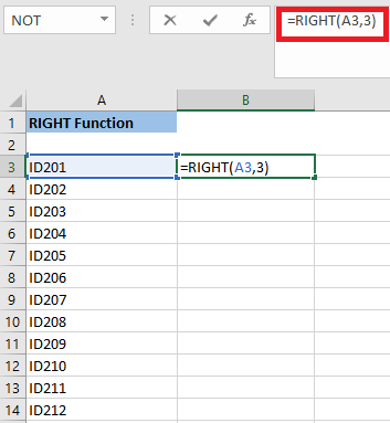
Example 3: In this example, we have a list of IDs such as "ID201," "ID202", "ID203". "ID204," etc., in column A. 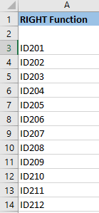
In this case, the last three digits of the ID are unique, and the text "ID" is redundant. As a result, we'd like to eliminate "ID" form the list of identifiers. We will apply the below formula: =RIGHT(A3,3)
The RIGHT function returns 210 in cell B3. Using the same procedure, we will extract the last three digits of each ID. 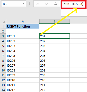
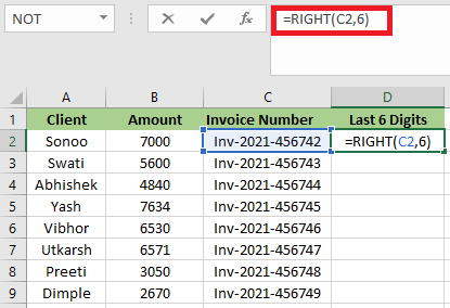
Example 4: In this example, we have a dataset that contains invoice numbers. We want to extract the last 6 digits of each of the invoice numbers so, to do this, we have to use the RIGHT function. 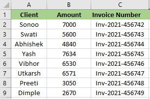
Using Excel's RIGHT function, we can extract the last 6 digits of the above text. =RIGHT(C2,6)
After applying the RIGHT function, the result will be: 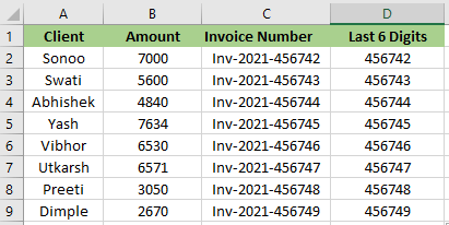
Example 5: Suppose we have serial numbers ranging from A2 to A13, and we want to extract 8 characters from the right. 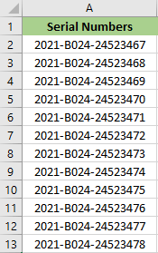
The RIGHT function returns the last 8 digits from the text's right end. 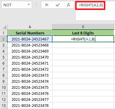
After applying the formula, the result will be: 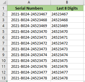
Example 6: In this example, we have the name of two animals in column A. Using comma and space, the names are separated, as shown in the below screenshot. We need to extract the last name. 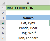
In order to extract the last name, we have to use the following RIGHT formula. =RIGHT(A4,LEN(A4)-FIND(" ",A4))
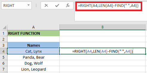
"Lynx" is the output of the RIGHT formula. The output for the remaining cells is also found in the same way. Example 7: Excel's RIGHT function does not work with dates. Because the RIGHT function is a text function, it can also extract numbers, but it cannot extract dates. Let's say cell A2 has a date "1-sept-2021". 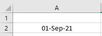
Now, we will try to extract the year with the help of the RIGHT formula. 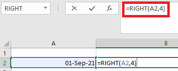
The result would be 4440. 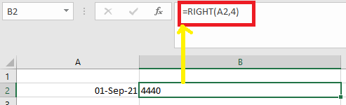
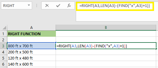
In excel. Ideology 4440 means 2021 if the format is in Dates. As a result, Excel's RIGHT function will interpret it as a number rather than a date. Example 8: In this example, we have 2-Dimensional data. The length is multiplied by the width, as we can see in the below screenshot. We need to extract the width from the given dimension. 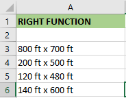
We will use the following RIGHT formula for the first dimension. =RIGHT(A3,LEN(A3)-FIND("x",A3)+1))
The RIGHT formula returns "700 ft" for the first dimension. We have to drag the fill handle to determine the results of the other cells. 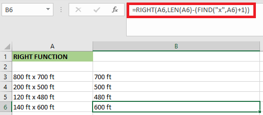
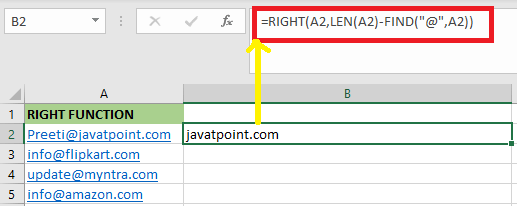
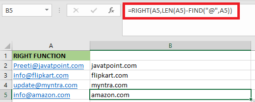
Example 9: In this example, we have a list of email addresses. We need to extract the domain name from these email IDs. 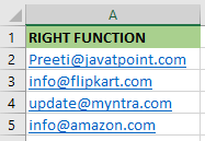
In order to extract the domain name from the first email address, we have to use the below RIGHT formula. =RIGHT(A2,LEN(A2)-FIND("@",A2))
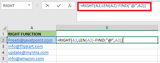
The length of the string A2 is given by "LEN(A2)". It will return 21.
Example 10: In this example, there are some errors that we may encounter while using the web-based software are listed below. We have to extract substring after the last occurrence of the delimiter. 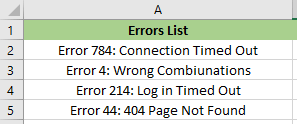
We can do this by using the combination of LEN, SEARCH and SUBSTITUTE along with the RIGHT function in Excel. 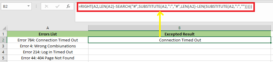
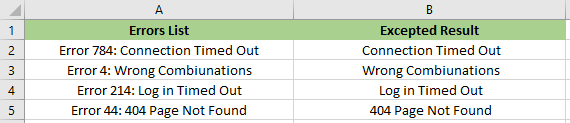
After applying the above formula, the result would be: LEN(A2)-LEN(SUBSTITUTE(A2,":",""))
Things to Keep in Mind When Using the RIGHT Function:The following are the things which we have to keep in mind when using RIGHT function:
Next TopicNOT Function in Excel
|
 For Videos Join Our Youtube Channel: Join Now
Feedback
- Send your Feedback to [email protected]
Help Others, Please Share


