| |

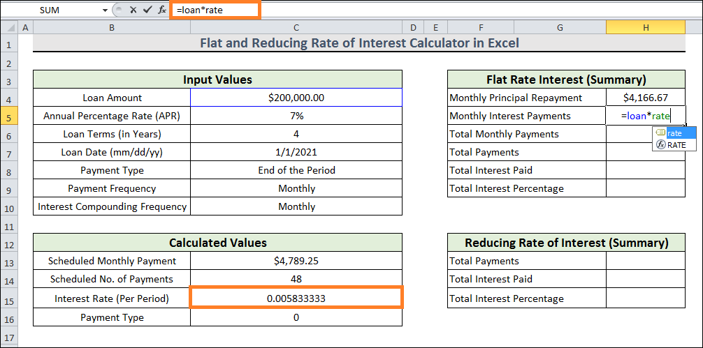
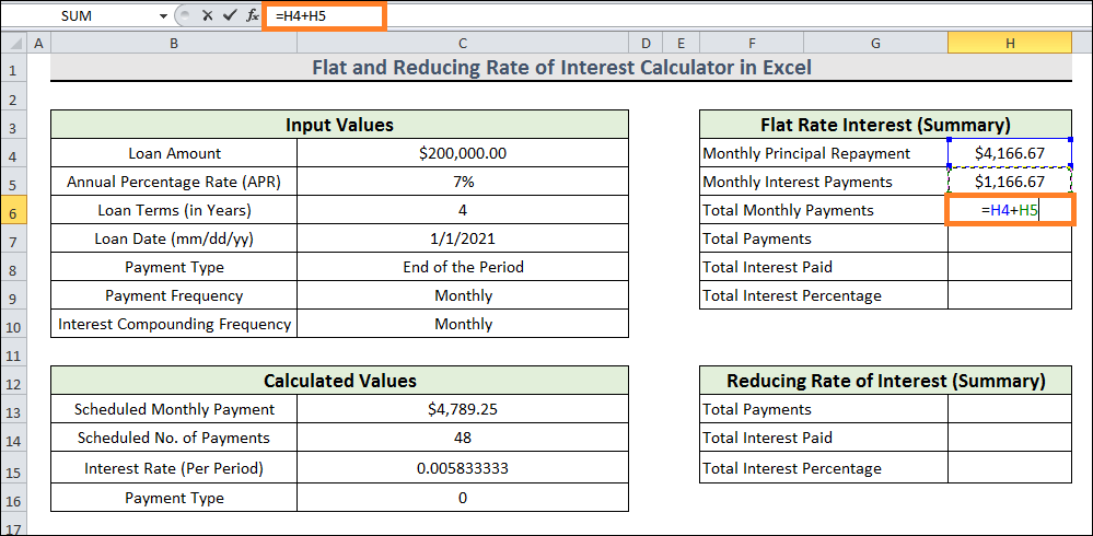
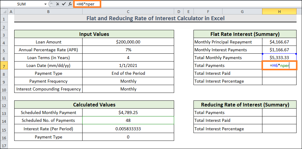
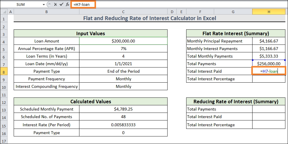
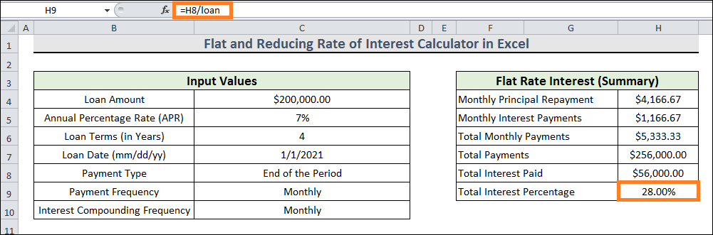
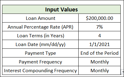
Reducing Rate of Interest Calculator with Flat in ExcelIn this tutorial, we'll guide you through creating an Excel calculator that calculates reducing interest rates with flats rates in a few simple steps. You can use the Calculator to see what methods provide a higher financial return. So, let's dive right into the content, without any delay. Flat Rate of InterestThe terms "reducing balance rate" and "flat rate interest" are unfamiliar to many people in the financial world. Being in the dark when handling your finances is not a good idea. Financial catastrophes can result from a lack of understanding of fundamental finance concepts. After completing this tutorial, these two phrases will be clear to you. Additionally, you will receive an Excel calculator with a flat and decreasing interest rate. First, let's look at the formula used to determine the flat interest rate. An example will help you better comprehend this definition. Say you borrowed $200,000 at a six per cent annual percentage rate (APR). You have five years to repay the debt and must make an instalment payment each month. ($200,000 x 4 x 7%) / 48 will be your flat rate interest. You will pay your interest on this each time you make an instalment. Let's compute your principal repayments now. The result of plugging in the numbers is = $200,000 / 48. Thus, your monthly payment total will be $4,166.67+ $1,166.67= $5,333.33.The following figure shows a summary of the computation done above utilizing my flat rate interest calculator. In addition, the Calculator displays the following data: The entire amount paid: $256,000.00 $56,000.00 was paid in interest overall. For the next five years, you will be paying an interest rate of 28% per cent. Do you realize that the rate is high? Reducing Interest RateBanks and other financial organizations extensively use this strategy because it offers a more efficient way to manage loans. Using the loan information provided above, let's determine the decreasing interest rate.
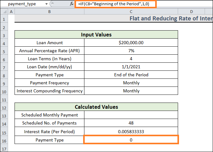
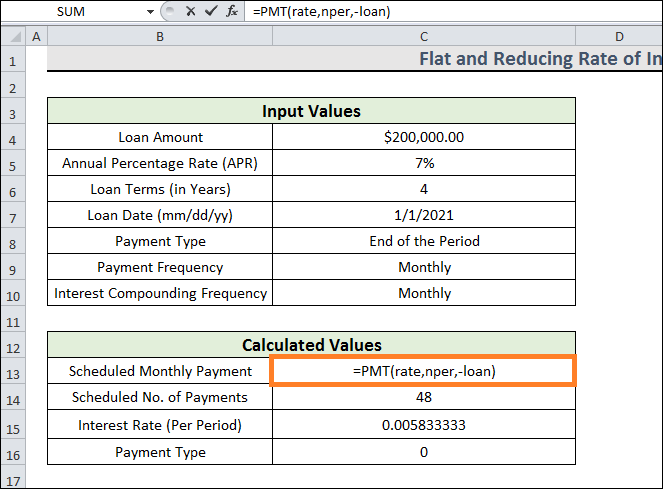
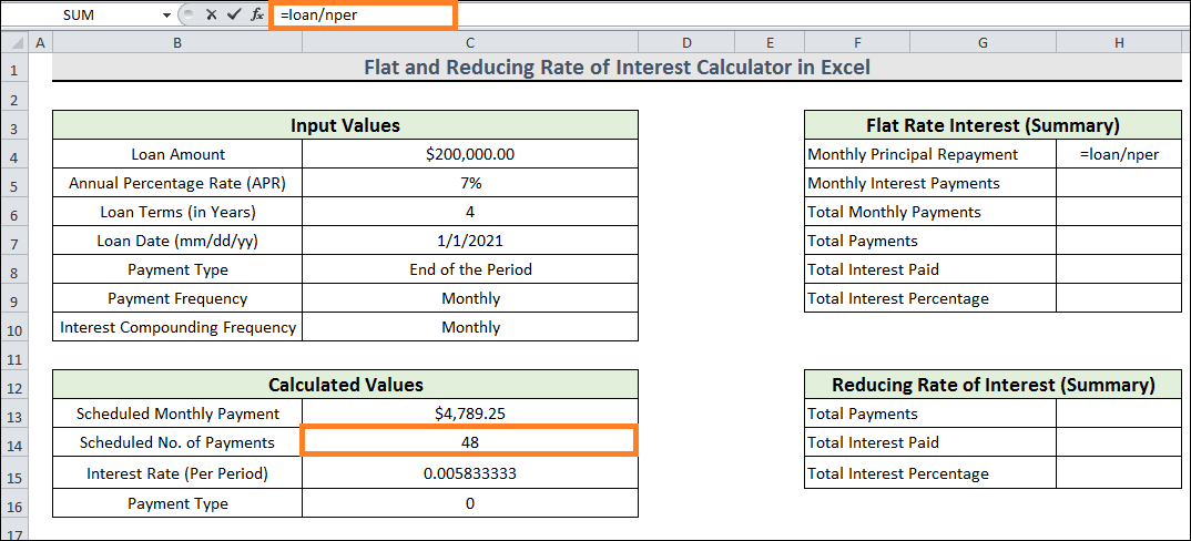
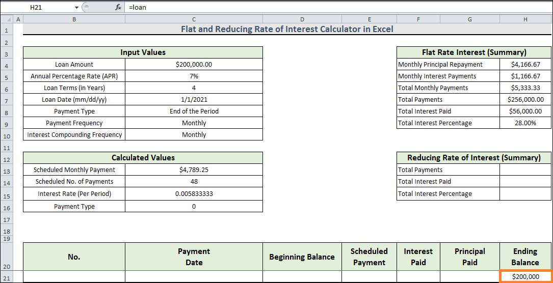
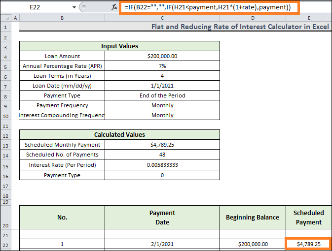
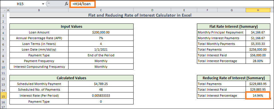
The monthly rate must first be determined if the frequency of payments is monthly: The next step is to use Excel's PMT function to determine the loan's monthly PMT: This time, the numbers are as follows: rate = 0.005833333 nper = 48; [nper = total number of periods];-loan = -200,000; [loan equals negative since we want the PMT to be positive]. $4789.25 is the value that it returns. 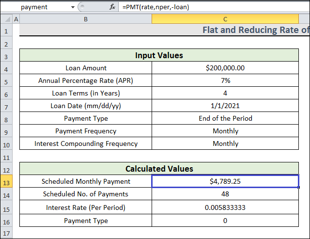
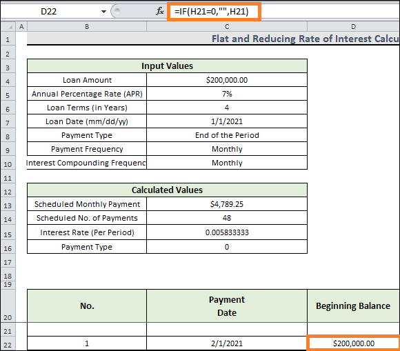
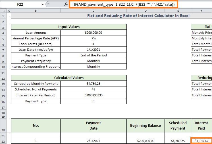
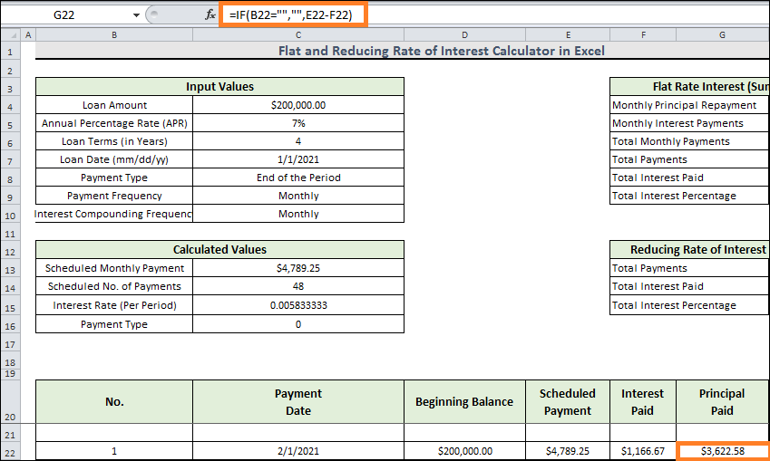
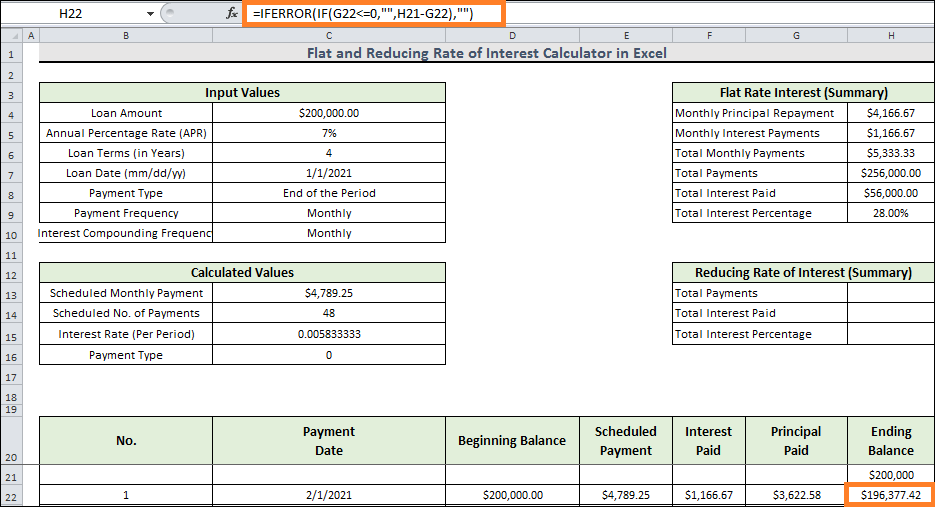
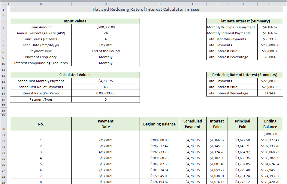
Let's now talk about how the entire thing operates: First Month:You simply take out the loan at the beginning of the first month. That leaves a $200,000 balance. You are responsible for paying the financial institution $4789.25 (the PMT payment) at the end of the initial month. What percentage of this sum ($4789.25) is interest paid? The interest for the first month is $1166.67 ($200,000 x 0.005833333). Therefore, $1166.67 of the $4789.25 total is given as interest. You will be refunded $4789.25 less $1166.67 or $4789.25 as a portion of your principal. Your new principal, therefore, will be as follows at the end of the first month: $200,000 - $3,622.58= $196377.42. Second Month:At the beginning of the second month, $196,377.42 is your new principal. By the conclusion of the second month, you are giving the financial institution $4789.25, which is the PMT amount. To what extent is interest paid on this sum ($4789.25)? The interest for the second month is $196,377.42 x 0.005833 = $1145.5324. Therefore, the interest payment is $1145.5324 out of $4789.25. Your principal will be reduced by the remaining amount, which is $4789.25- $1145.53= $3643.72. Consequently, your new principal after the second month will be $196,377.42 - $3643.72= $192,733.7. That's how the entire procedure moves forward. You can see the entire procedure in the following pictures. 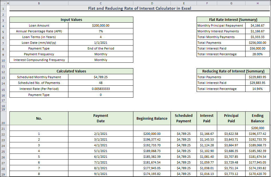
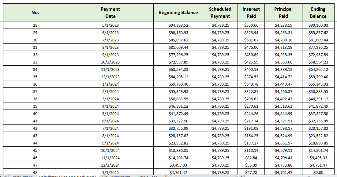
The graphic below illustrates how, at the most recent payment, we only paid $27.78 towards interest and used the remaining $4,761.47 to pay down our principal. We have 0.00 as our final balance. Therefore, that is our final payment to the bank. See, using a loan with a decreasing interest rate is easy. The total interest we pay on this system is only 14.94% at the end of the day. 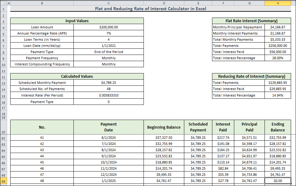
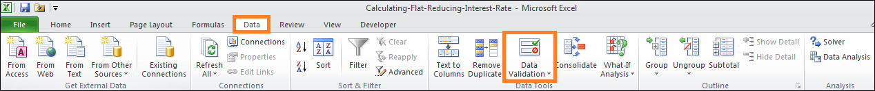
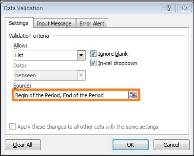
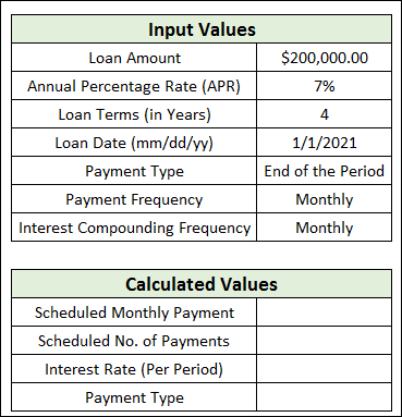
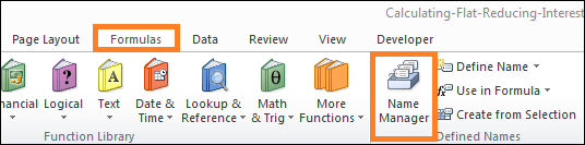
Excel Calculator with Step-by-Step Instructions for Reducing Interest RateHere are four easy steps to develop an Excel calculator for flat and reducing interest rates. First, all of the necessary values will be entered. The interest rate on a flat rate will then be determined. The payment schedule will be located third. We will complete the steps by calculating the lowering rate of interest. First, input the necessary values. This initial step will involve typing the necessary values. We will employ data checking to further enable users to set the data through a dropdown list. In the data validation dialogue box, we will enter the permitted values in the source field, separated by commas.
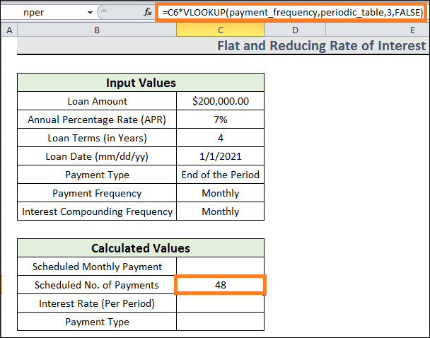
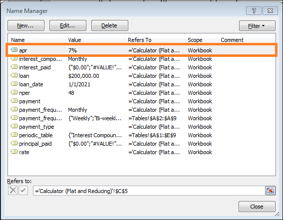
Identifying Flat Rate Interest The flat rate of interest will be determined in this second step. The functions VLOOKUP, PMT, and IF will be used. We are also using the name range to make things easier to apply. For the VLOOKUP function's lookup range, we have utilized a table. To prevent accidental value changes by users, this table is hidden.
Formula Explanation
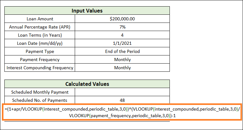
Formula Explanation
Result: 12.
Result: 12.
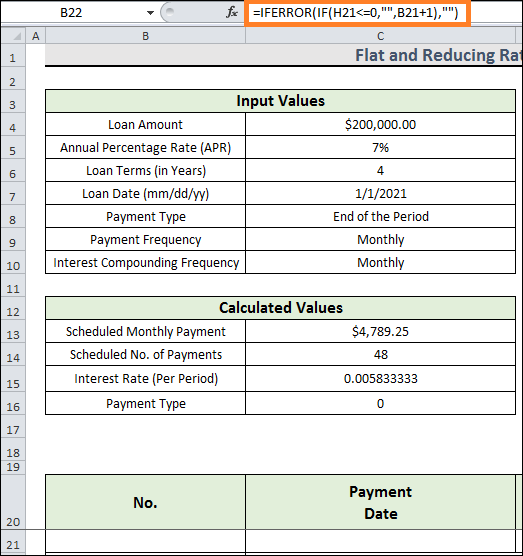
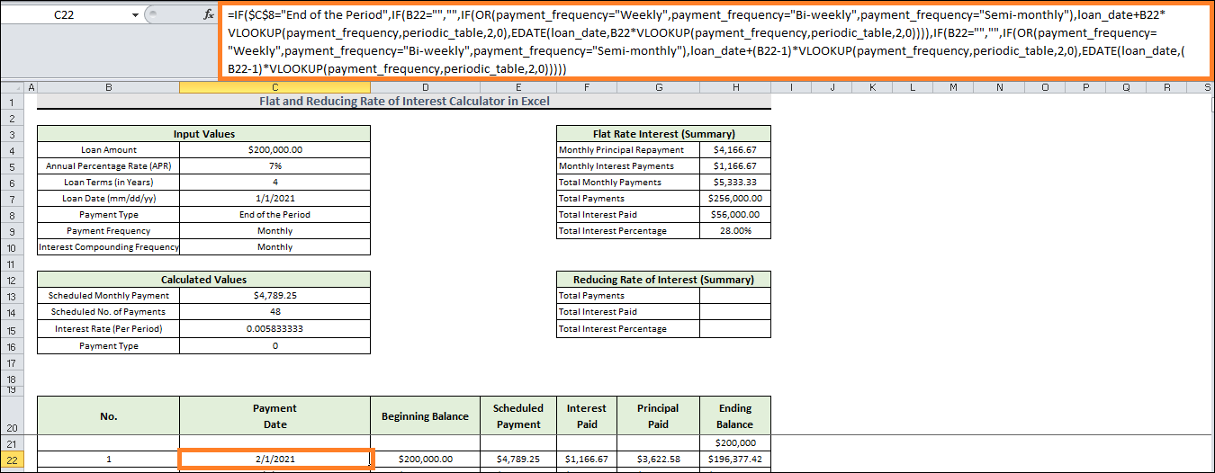
Compute the Payment Schedule This third stage is where we'll figure out the payment plan. In this stage, the AND, OR, EDATE, & IFERROR functions are the four new functions we will use. Let us dive right into the procedures.
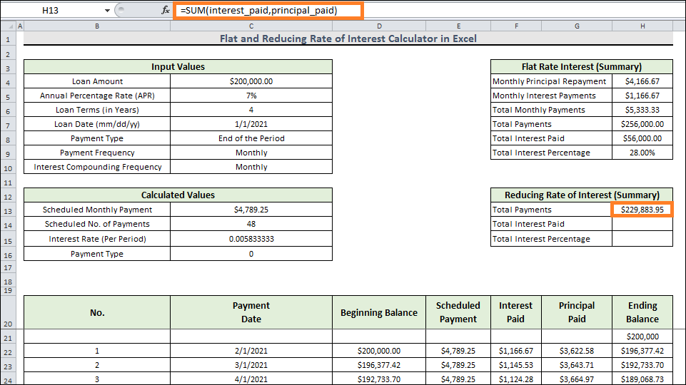
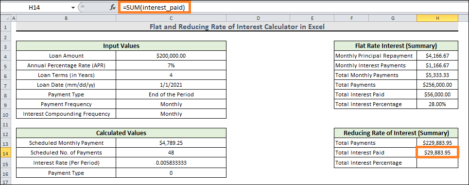
Determine the Interest Rate Reduction In this final phase, we will determine the rate of reduction of interest. In this phase, the SUM function will be utilized. Furthermore, the cell ranges F22:F10971 and G22:G10971 have been designated in the interest_paid and principal_paid, respectively.
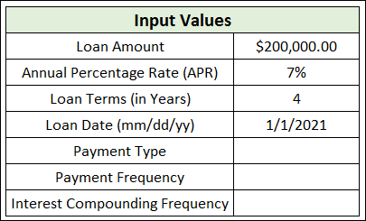
Instructions to follow while using this CalculatorThis Calculator is incredibly simple to use. In this part, we'll walk you through the values you must enter and adjust. To use this Calculator, enter the following values:
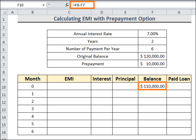
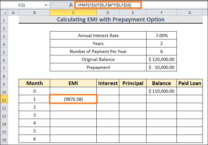
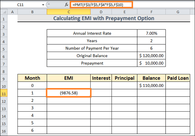
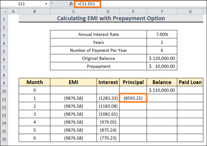
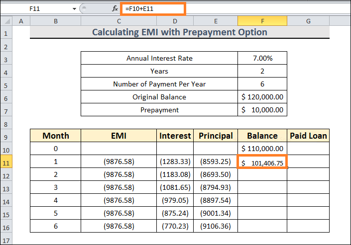
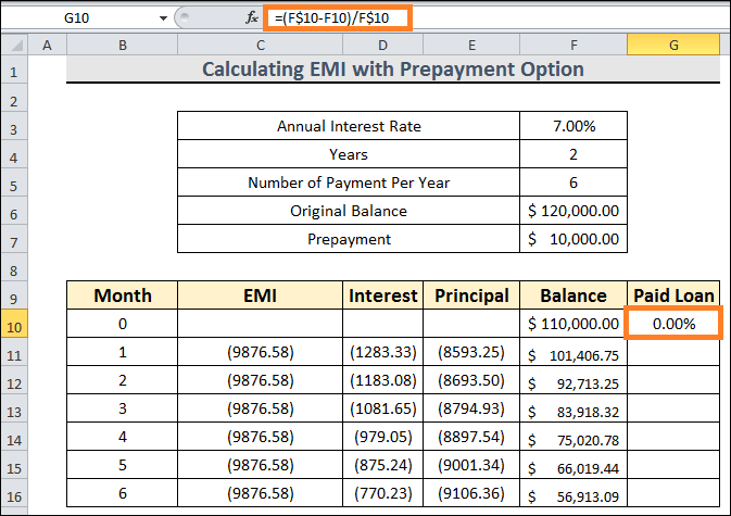
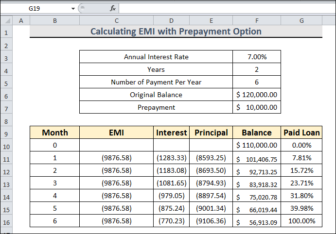
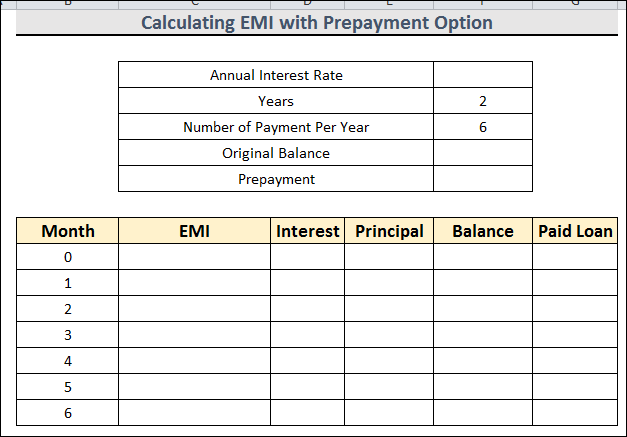
No more variables need to be entered. The Calculator will do the remaining job. Excel sheet featuring an EMI calculator with a prepayment optionAssume we have an Excel spreadsheet with the details of the EMI computation and a prepayment option. We will use Excel's PMT and IPMT finance algorithms to determine the EMI from our dataset with the prepayment option. PMT is a payment, while interest on payment is obtained using IPMT. With an Excel sheet with a prepayment option, we will use these financial tools to create the EMI calculator. Steps:
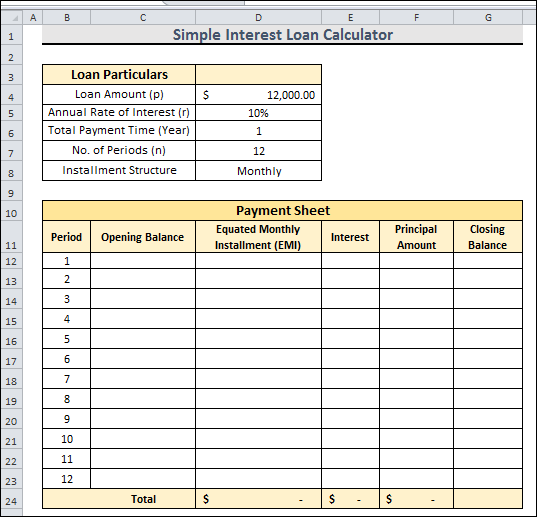
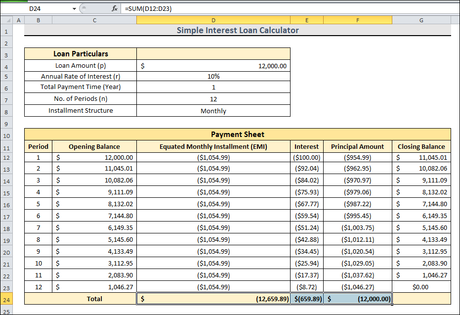
Simple Interest Loan Estimator with Excel FormulaSimple interest is the amount calculated from the principal of a bank loan or the first deposit made into a bank savings account. Another way to put it is the amount of interest, which immediately increases from the principal. Simple interest can be expressed mathematically as follows: The following are indicated by the symbols in this case:
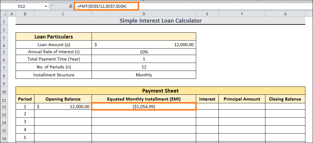
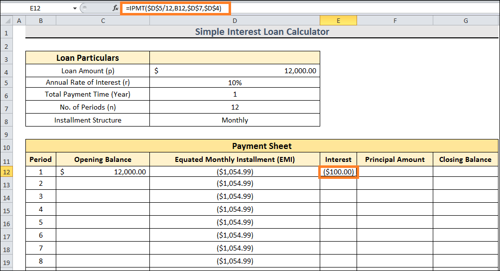
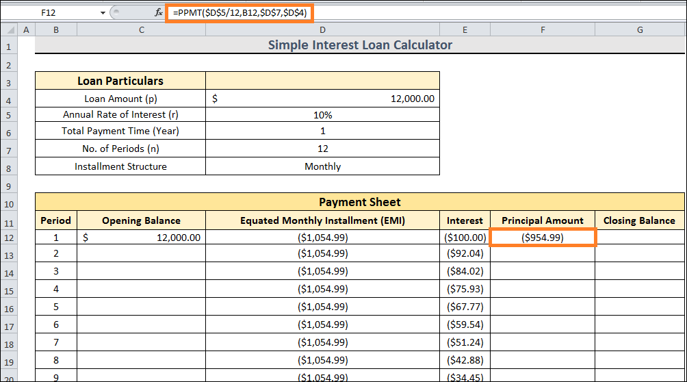
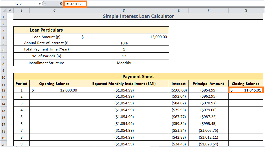
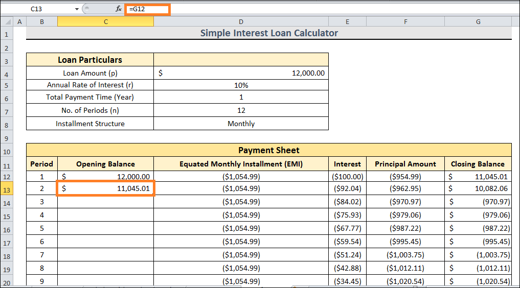
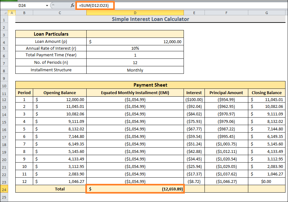
Now, we'll guide you through three appropriate instances of using Excel formula to create a basic interest loan calculator. This section will compute the primary amount using the PPMT function. Steps:
Conclusion:In conclusion, in the above tutorial, we learned the step-by-step process of creating Excel calculators to calculate reducing interest rates. We have covered various key concepts, and different tools for managing loans efficiently and have demonstrated the process of calculator creation. With Excel functions like VLOOKUP, PMT, IPMT, and PPMT, you can customize these calculators to fit your financial needs, making informed decisions with sureness. Whether for finance specialists, business professionals, or individuals managing their loans, this tutorial serves as a valuable resource for learning and implementing financial calculations in Microsoft Excel.
Next TopicCUSTOM LIST
|
 For Videos Join Our Youtube Channel: Join Now
Feedback
- Send your Feedback to [email protected]
Help Others, Please Share


