| |

Continuous Value PredictionTopicsThe file attached includes the following topics and sub-topics 1. Elements In Machine Learning
2. Regression
3. Regression Types In Detail
4. Conclusion Now, let us Dive Deep into Every Topic MachineLearningMachine Learning is all about making a machine learn as humans do. There are many techniques involved which help us to train the model and work accordingly as required. ElementsInMachineLearningHere are some essential machine-learning ideas and elements:
With several applications in different sectors of the economy, including marketing, banking, and healthcare, machine learning is a rapidly developing field. It can fundamentally alter how we handle and apply data in order to tackle challenging issues and come to wise judgments. RegressionFor modeling and analyzing the relationships between variables, Regression is a fundamental statistical and machine-learning tool. It is mostly used to forecast a continuous outcome variable (dependent variable) from one or more input factors (independent variables), which might be continuous or categorical. 
Finding the best-fit line or curve that illustrates the relationship between the independent factors and the dependent variable is the main objective of regression analysis. The regression model is the name given to this line or curve. Once the model has been trained on historical data, it can be applied to forecast new data or estimate the values of the dependent variable. Regression'sPrimaryFeaturesAreAsFollows:Let us look at some of the features of Regression and the types involved in the topic regression VariousRegressions: First, let us look at different types of Regression 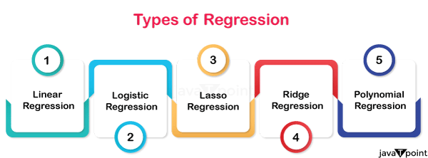
1. LinearRegression:
2. MultipleLinearRegression:
3. PolynomialRegression:
4. LogisticRegression:
ModelAssessment:
Assumptions:
Applications:
Regularisation:
Regression analysis is a potent method for deriving insights from real-world information, analyzing and modeling relationships within data, and making predictions. It has numerous applications in a wide range of fields, including statistics and machine learning. RegressionTypesInDetailLet us look at each Regression type deeply so that we get a better understanding of each Regression model. 1. SimpleLinearRegressionSimple Linear Regression is a statistical technique that involves fitting a linear equation to the observed data in order to represent the relationship between a single dependent variable (goal) and a single independent variable (predictor or feature). The independent and dependent variables are assumed to have a linear relationship. The model equation has the following form: Y = B₀ + B₁X + ε Where: The aim (dependent variable) is Y. The independent variable (feature or predictor) is X. The intercept (the value of Y when X is 0) is equal to B0. The slope, or the amount that Y varies for a unit change in X, is B1. The error term (the discrepancy between the actual and expected values) is represented by the symbol. Simple linear Regression, sometimes referred to as the least squares method, seeks to predict the values of B0 and B1 that minimize the sum of squared errors (SSE). FormulasForSimpleLinearRegression: Let us look at some of the most important formulas that are used while working on linear Regression.
Example: Let's go over a straightforward example of simple linear Regression to forecast a student's final exam grade (Y) based on the quantity of study time they put in (X). Assume you have the dataset shown below:
1. Calculate the means of X and Y: Mean(X) = (2 + 3 + 4 + 5 + 6) / 5 = 4 Mean(Y) = (65 + 75 + 82 + 88 + 92) / 5 = 80.4 2. Calculate the slope (β₁) using the formula: β₁ = Σ((Xᵢ - Mean(X)) * (Yᵢ - Mean(Y))) / Σ((Xᵢ - Mean(X))² β₁ = ((2-4)(65-80.4) + (3-4)(75-80.4) + (4-4)(82-80.4) + (5-4)(88-80.4) + (6-4)*(92-80.4)) / ((2-4)² + (3-4)² + (4-4)² + (5-4)² + (6-4)²) β₁ ? 5.52 3. Calculate the intercept (β₀) using the formula: β₀ = Mean(Y) - β₁ * Mean(X) β₀ ? 80.4 - 5.52 * 4 β₀ ? 57.28 4. The linear regression equation is: Y = 57.28 + 5.52X Now, based on the quantity of study time, you can apply this equation to forecast your final exam results. By including a regularisation element in the linear regression equation, the Ridge Regression and Lasso Regression procedures in linear Regression address the issue of multicollinearity and guard against overfitting. A description of both methods, along with their formulas and illustrations, is provided below: RidgeRegression: By including a regularisation element in the linear regression equation, the Ridge Regression and Lasso Regression procedures in linear Regression address the issue of multicollinearity and guard against overfitting. A description of both methods, along with their formulas and illustrations, is provided below: Ridge Objective Function = SSE (Sum of Squared Errors) + λ * Σ(βᵢ²) Where: When performing simple linear or multiple linear Regression, SSE, or Sum of Squared Errors, is used. The regularisation parameter, or λ (lambda), regulates the regularization's degree of strength. The total of the squared coefficients is denoted by Σ(βᵢ²). Ridge Regression attempts to reduce this objective function. 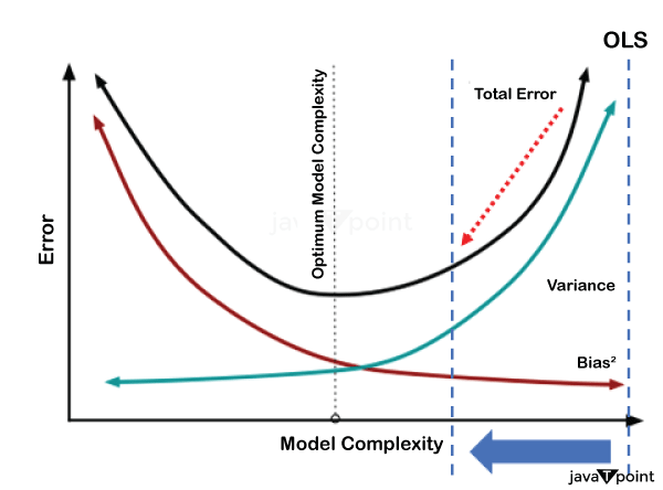
Example: Assume you are using Ridge Regression to forecast home prices using two predictors: square footage (X1) and the number of bedrooms (X2). Similar to multiple linear Regression, the Ridge Regression equation also includes a regularisation term: Y = β₀ + β₁X₁ + β₂X₂ + λΣ(βᵢ²) This equation can be used to minimize the objective function while estimating the coefficients β₀, β₁, and β₂. LassoRegression: Another method that includes a penalty element in the linear regression equation is called Lasso Regression, sometimes referred to as L1 regularisation. Lasso, in contrast to Ridge Regression, promotes model sparsity by bringing some coefficients to a precise zero value. The Lasso Regression's updated objective function is as follows: Lasso Objective Function = SSE + λ * Σ|βᵢ| Where: When performing simple linear or multiple linear Regression, SSE, or Sum of Squared Errors, is used. The regularisation parameter, denoted by λ (lambda), regulates the degree of regularisation. The total of the absolute values of the coefficients is shown by the symbol Σ|βᵢ|. Lasso regression attempts to reduce this objective function to the minimum while potentially reducing some coefficients to zero. 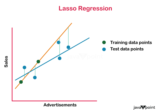
Example: The Lasso Regression equation is as follows, using the same example of forecasting house prices with square footage (X1) and the number of bedrooms (X2) as predictors: Y = β₀ + β₁X₁ + β₂X₂ + λΣ|βᵢ| This equation can be used to minimize the objective function while estimating the coefficientsβ₀, β₁, and β₂. Some of the coefficients could be set exactly to zero via Lasso, choosing only the most crucial predictors for the model. In real life, the regularisation parameter is set to a value that optimally balances model complexity and goodness of fit using methods like cross-validation. For managing multicollinearity and avoiding overfitting in linear regression models, Ridge and Lasso Regression are useful methods. 2. MultipleLinearRegressionAn expansion of simple linear Regression, multiple linear Regression involves fitting a linear equation to the observed data to represent the relationship between a dependent variable (the target) and two or more independent variables (predictors or characteristics). The model's equation has the following form in multiple linear Regression: Y = β₀ + β₁X₁ + β₂X₂ + ... + βₚXₚ + ε Where: The aim (dependent variable) is Y. The independent variables (predictors or characteristics) are X1, X2,..., and Xp. The intercept is β₀. The coefficients of the independent variables are β₀, β₁, β₂, …. βₚ The error term (the discrepancy between the actual and expected values) is represented by the symbol. Similar to simple linear Regression, the objective of multiple linear Regression is to estimate the values of β₀, β₁, β₂, …. βₚ that minimize the sum of squared errors (SSE). 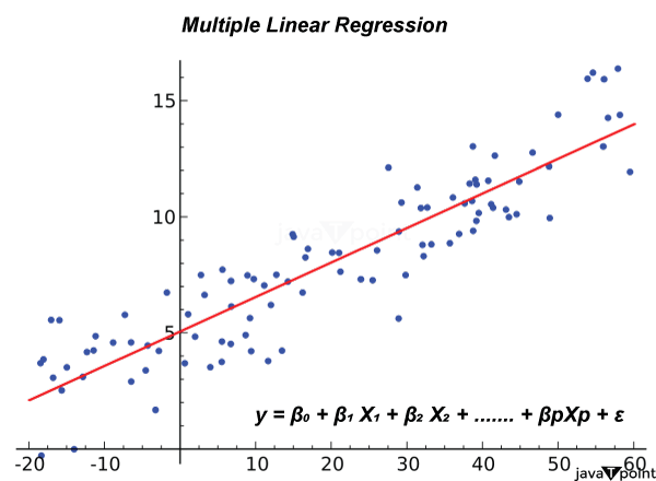
FormulasForMultipleLinearRegression:
Example: Let's look at an illustration of multiple linear Regression to forecast the cost of a home (Y) based on two independent variables: the home's square footage (X1) and the number of bedrooms (X2). Assume you have the dataset shown below:
Calculate the means of X₁, X₂, and Y: Mean(X₁) = (1500 + 2000 + 1800 + 2200 + 1600) / 5 = 1820 Mean(X₂) = (3 + 4 + 3 + 5 + 4) / 5 = 3.8 Mean(Y) = (200,000 + 250,000 + 220,000 + 280,000 + 210,000) / 5 = 232,000 Estimate the coefficients (β₀, β₁, β₂) using the formulas: β₀ (intercept) = Mean(Y) - (β₁ * Mean(X₁) + β₂ * Mean(X₂)) β₁ (coefficient for X₁) and β₂ (coefficient for X₂) are calculated similarly using the formula for each. The multiple linear regression equation is: Y = β₀ + β₁X₁ + β₂X₂ This equation can now be used to anticipate property prices depending on square footage and the number of bedrooms. (4-4)(82-80.4) + (5-4)(88-80.4) + (6-4)*(92-80.4)) / ((2-4)² + (3-4)² + (4-4)² + (5-4)² + (6-4)²) β₁ ? 5.52 5. Calculate the intercept (β₀) using the formula: β₀ = Mean(Y) - β₁ * Mean(X) β₀ ? 80.4 - 5.52 * 4 β₀ ? 57.28 6. The linear regression equation is: Y = 57.28 + 5.52X Now, based on the quantity of study time, you can apply this equation to forecast your final exam results. By including a regularisation element in the linear regression equation, the Ridge Regression and Lasso Regression procedures in linear Regression address the issue of multicollinearity and guard against overfitting. A description of both methods, along with their formulas and illustrations, is provided below: 3. PolynomialRegressionRegression analysis that uses nth-degree polynomials to represent the relationship between the independent (predictor) and dependent (target) variables is known as polynomial Regression. This type of linear Regression uses polynomial equations to represent the relationship between the variables rather than linear equations. Regression using polynomials is very helpful when there is a curved pattern rather than a straight line between the variables. The definition of polynomial Regression, along with its formula and an illustration, are given below: FormulaForPolynomialRegression: The equation for polynomial Regression is as follows: Y = β₀ + β₁X + β₂X² + β₃X³ + ... + βₙXⁿ + ε Where: The aim (dependent variable) is Y. X is a predictor that is an independent variable. The coefficients of the polynomial terms are β₀, β₁, β₂, β₃, ..., βₙ. The highest power of X employed in the equation is determined by the polynomial's degree, n. The error term (the discrepancy between the actual and expected values) is represented by the symbol. Similar to linear Regression, polynomial Regression aims to estimate the values of the coefficients β₀, β₁, β₂, β₃, ..., βₙ that minimize the sum of squared errors (SSE). 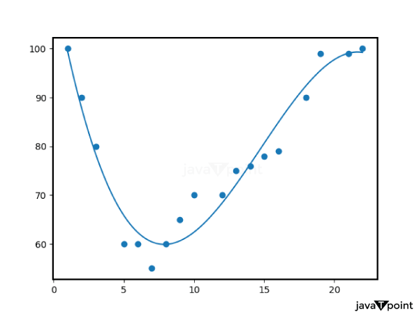
Example: Let's look at an instance where you need to forecast the relationship between an individual's income (Y) and their number of years of work experience (X). The link is not linear because, with more years of experience, salaries tend to rise faster. A polynomial regression may be a good option in this situation. Assume you have the dataset shown below:
If you use a polynomial with a degree of 2, for example, you will fit a quadratic equation when using polynomial Regression: Assume you have the dataset shown below: Y = β₀ + β₁X + β₂X² + ε Now, while minimizing the SSE, use this equation to estimate the coefficients β₀, β₁, and β₂. This Regression can be carried out using a variety of statistical or machine-learning approaches, such as gradient descent or specialized regression libraries in Python or R. Using the polynomial equation, you can make predictions after estimating the coefficients. For illustration, the following would be the compensation range for a person with six years of experience: Incorporate X = 6 into the formula: Y = β₀ + β₁(6) + β₂(6²) To calculate Y, substitute the predicted coefficients. In order to avoid overfitting or underfitting the data, it's crucial to select the right degree of the polynomial. Polynomial Regression is a versatile technique that may capture non-linear correlations between variables. 4. LogisticRegressionIt is feasible to predict categorical outcomes with two possible values, commonly expressed as 0 and 1 (for example, yes/no, spam/not spam, pass/fail), using the statistical method known as logistic Regression. Contrary to what its name implies, Logistic Regression is a classification algorithm. Utilizing the logistic function to translate predictions to a probability between 0 and 1, it represents the likelihood that an input belongs to a specific class. The definition of logistic Regression, along with its formula and an illustration, are given below: FormulaForLogisticRegression: The logistic (or sigmoid) function is used in the logistic regression model to simulate the likelihood that the dependent variable (Y) will be 1 (or fall into the positive class): P(Y=1|X) = 1 / (1 + e^(-z)) Where: The probability that Y is 1 given the input X is known as P(Y=1|X). The natural logarithm's base, e, is about 2.71828. The predictor variables are combined linearly to form z: z = β₀ + β₁X₁ + β₂X₂ + ... + βₚXₚ The coefficients for the predictor variables X1, X2,..., Xp are β₀, β₁, β₂, ..., βₚ . For modeling probabilities, the logistic function makes sure that the result is confined between 0 and 1. You normally select a decision threshold (like 0.5) to categorize the input into one of the two classes. If P(Y=1|X) is larger than the threshold, the input is categorized as 1; otherwise, it is categorized as 0. 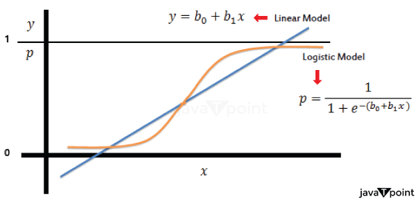
Example: Let's look at an illustration where you want to forecast a student's exam result based on how many hours they studied (X) and whether they will pass (1) or fail (0). Assume you have the dataset shown below:
In order to forecast whether a student who puts in a specific amount of study time will pass or fail, you should create a logistic regression model.
For binary and multi-class classification issues, the classification algorithm known as logistic Regression is frequently employed in machine learning. When modeling the likelihood of an event occurring based on one or more predictor factors, it is especially helpful. ConclusionA fundamental method for modeling and predicting continuous outcomes based on the connections between variables in machine learning is Regression. It includes a range of methods, including straightforward linear Regression and more intricate ones like polynomial Regression, ridge, and lasso regression. These techniques give us the ability to measure and analyze the influence of predictor factors on the target variable, offering important insights into a variety of fields, including finance, healthcare, marketing, and more. Because of how easily they can be understood, regression models are highly valued as tools for both comprehending data relationships and making predictions. In addition, thorough feature engineering and data pretreatment are frequently needed for regression approaches to produce reliable findings. Regression's crucial model selection and evaluation processes involve picking the best regression strategy and validating it with metrics like MSE and R2. Regression is a flexible and broadly applicable method in the machine learning toolkit that enables data scientists and analysts to create prediction models that improve decision-making processes in a variety of domains.
Next TopicBayesian Regression
|
 For Videos Join Our Youtube Channel: Join Now
Feedback
- Send your Feedback to [email protected]
Help Others, Please Share


