| |

Python - Poisson Discrete Distribution in StatisticsOne of the fundamental concepts in statistics is the study of random variables and their distributions. This tutorial gives you a thorough understanding of Poisson Discrete Distribution, which is a key component in statistics/probability theory, and finally, learn about its various properties and calculations using Python. Let us start the discussion by understanding the random variable terms involved: Random VariableA random variable is an outcome of a random experiment. It is a numerical quantity whose values belong to the set of possible outcomes of random experiments or events. For example:
The random variable can be categorized into two types:
Poisson Discrete DistributionThe Poisson distribution is a discrete probability distribution that expresses the probability of a given number of events occurring in a fixed interval of time or space. A discrete probability distribution is the probability distribution of a random variable that can take on only a countable number of values. - Wikipedia It's often used to describe rare and random events, such as the number of phone calls received at a call center in a given hour, the number of accidents at an intersection in a day, or the number of emails received per hour. Key Characteristics of the Poisson Distribution:
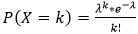
Probability Mass FunctionThe probability mass function assigns a probability to each possible value of a random variable. The probability mass function (PMF) of the Poisson distribution is given by: 
Where:
You might find different symbols representing the pmf formula on different sources, so don't get confused. Let's explore the Poisson distribution with a couple of examples: Example 1: Phone Calls at a Call Center Suppose a call center receives an average of 5 calls per hour. What is the probability of receiving exactly 3 calls in the next hour? Here, λ = 5 (average rate of calls per hour) and k = 3 (desired number of calls). Putting these values into the Poisson PMF formula: So, the probability of receiving exactly 3 calls in the next hour is approximately 0.14037, or about 14.04%. How to Calculate Probabilities using Poisson Distribution in Python?To calculate the probability using Poisson distribution, we have 'scipy.stats.poisson.pmf' function which is part of SciPy library. This function is used to calculate the probability of observing a specific value "k" from the distribution. Syntax: Parameters:
In the above example, it is given that the average number of calls = 5 per hour and we need to find the probability of getting exactly three calls in the next hour. Output: Poisson PMF: 0.1403738958142805 The above output is equal to what we calculated manually. Example 2: Accidents at a Crossroad Suppose a Crossroad experiences an average of 2 accidents per day. What is the probability of having at least 4 accidents and, at most 6 accidents in a day? Here, λ = 2, and we want to find P(X ≥ 4 and X<=6), which is the sum of probabilities for having 4, 5, and 6 accidents. Calculating each probability and summing them up: So, the probability of having at least 4 and, at most 6 accidents in a day is approximately 0.1383, or about 13.83%. Python Code: Output: Poisson PMF: 0.13834273397520408 How to Generate Poisson Distribution?Method 1 - Using NumPyLet's create a random (1 x 15) distribution with λ = 3. Here, we started with importing the random method from the NumPy module. This line returns a list containing 15 random samples from the Poisson distribution. We pass lam=3, meaning the average number of occurrences of an event is 3. Each number in the array represents the number of events occurring in a fixed interval of time. When we run the program, we get the output: Poisson Distribution: [4 1 7 2 3 4 4 3 3 7 7 5 2 2 0] In this output, each number represents the number of events occurring in a fixed interval, and the distribution reflects the characteristics of the Poisson distribution with an average rate of 3. Method 2 - Using SciPyWe can use poisson.rvs(mu, size) to generate a Poisson distribution. Output: Poisson Distribution: [8 2 2 4 2 2 3 3 1 3 3 2 0 1 3] How to Plot Poisson Distribution?To plot the Poisson Distribution, we first need to create a sample. Here, we use scipy.stats.poisson.rvs() method to generate a random sample from the Poisson distribution and matplotlib library to plot a histogram. Output: 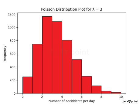
When we run this code, it generates a histogram representing the distribution of 5000 random numbers drawn from a Poisson distribution with a mean of 3. The histogram shows the frequency of occurrence of different values within the specified range, helping us visualize the shape of the Poisson distribution. Calculating Probabilities of each sample value:Output: 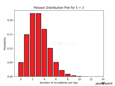
Explanation: In the above code, we first created a random sample from the Poisson distribution with mean = 3 and a sample size = 5000. We create a list `prob_dist` to store the probability of each value from the sample. We then use a for loop that calculates the probability mass function (PMF) for each value in the array 'x'. Finally, we display the bar chart, showing the Poisson distribution for the given parameters. The plot represents the probabilities of different numbers of accidents occurring per day, assuming an average rate of 3 accidents per day (λ = 3). We can also plot the Poisson Distribution with different mean values. Plot Poisson Distribution with λ = [2, 3, 4, 5]Output: 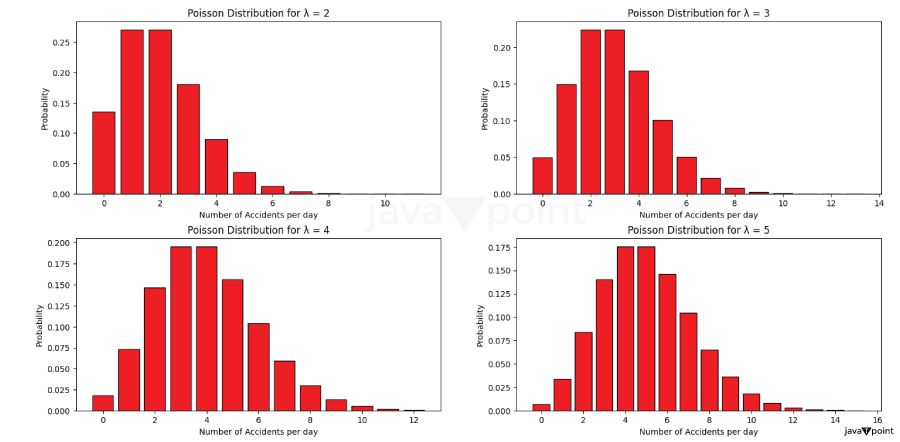
Explanation: In the above code:
It generates four distinct Poisson distribution subplots for different values of λ. Cumulative Distribution Function (CDF):Cumulative Distribution Function (CDF) describes the probability that a random variable takes on a value less than or equal to a specific value. Mathematically, the Cumulative Distribution Function of a random variable X is defined as: Where:
We can utilize the Poisson CDF function to compute the cumulative probability. Q. An email server receives an average of 6 emails per hour. What is the probability of receiving fewer than 5 emails in the next hour? Ans. Output: Probability using PMF P(X < 5) = 0.2850565003166312 Cumulative Probability of X < 5 = 0.2850565003166312 In this code: We set k to 4 because we want to find the probability of receiving fewer than 5 emails, which corresponds to the Poisson random variable X being less than 5.
The final result represents the probability of receiving fewer than 5 emails in the next hour. Below are some practice problems that you can solve. We encourage you to solve the problem independently before moving towards the given solution. Q. 1 A factory produces an average of 10 defective items per week. What is the probability of having exactly 8 defective items in a week? Sol. Average rate of occurrence, λ = 10 Value for which to calculate pmf, k = 8 Output: Poisson PMF: 0.11259903214902009 Q. 2 A website experiences an average of 500 visits per hour. What is the probability of having more than 600 visits in a randomly selected hour? Sol. Average rate of occurrence, λ = 500 Value for which to calculate pmf, k = 600 Output: Poisson PMF: 1.3566714436562893e-06 Q. 3 A restaurant serves an average of 15 vegetarian meals per lunchtime. What is the probability of serving exactly 10 vegetarian meals during lunchtime? Sol. Average rate of occurrence, λ = 500 Value for which to calculate pmf, k = 600 Output: Poisson PMF: 0.04861075082960534 Q. A car rental agency rents an average of 4 luxury cars per day. What is the probability of renting fewer than 3 luxury cars on a given day? Sol. Average number of cars, λ = 4 Number of cars for which to calculate cdf, k < 3 Output: Poisson CDF: 0.23810330555354436 Q. 5 A retail store receives an average of 12 customers per hour. What is the probability of having more than 15 customers in the next hour? Sol. Average number of Customers = 12 Number of customers for which we want to calculate CDF, k > 15 Output: Poisson CDF of attending customers <= 15: 0.7720245323035447 Poisson CDF of attending customers > 15: 0.22797546769645527 To be Summarize:
Throughout the article, we've provided Python code examples for calculating probabilities using the Poisson PMF and CDF functions. These examples illustrate how to work with Poisson distributions and apply them to real-world scenarios. |
 For Videos Join Our Youtube Channel: Join Now
Feedback
- Send your Feedback to [email protected]
Help Others, Please Share


