Implementation of Neural Network in Image Recognition

Our next task is to train a neural network with the help of previously labeled images to classify new test images. So we will use the nn module to build our neural network.

There are the following steps to implement the neural network for image recognition:

Step 1:

In the first step, we will define the class which will be used to create our neural model instances. This class will be inherited from the nn module, so we first have to import the nn package.

Our class will be followed by an init() method. In init() first argument will always self, second argument will be the number of input nodes which we will call, the third argument will be the number of nodes in the hidden layer, fourth argument will be the number of nodes in the second hidden layer and the last argument will be the number of nodes in the output layer.

Step 2:

In the second step, we recall the init() method for the provision of various method and attributes, and we will initialize the input layer, both the hidden layer and the output layer. One thing remembers that we will deal with the fully connected neural network. So

Step 3:

Now, we will make the prediction, but before it, we will import torch.nn.functional package, and then we will use the forward() function and place self as a first argument and x for whatever input we will try to make the prediction.

Now, whatever input which will be passed in forward () function will pass to the object of linear1, and we will use relu function rather than sigmoid. The output of this will feed as an input into our second hidden layer and the output of our second hidden layer will feed to the output layer and return the output of our final layer.

Note: We will not apply any activation function in the output layer if we are dealing with multiclass dataset.

Step 4:

In the next step, we will set up out model constructor. According to our initializer we have to set input dimensions, hidden layer dimensions and output dimensions.

The pixel intensity of the image will be fed to our input layer. Since each image is of 28*28 pixels which have a total of 784 pixels which will be fed into our neural network. So we will pass 784 as the first argument, we will take 125 and 60 nodes in the first and second hidden layer, and in the output layer, we will take ten nodes. So

Step 5:

Now, we will define our loss function. The nn.CrossEntropyLoss() is used for multi-class classification. This function is the combination of log_softmax() function and NLLLoss() which is a negative log-likelihood loss. We use cross-entropy whatever training and classification problem with n classes. As such, it makes use of log probabilities, so we pass in the row output rather than the output of a softmax activation function.

After that, we will use the familiar optimizer, i.e., Adam as

Step 6:

In the next step, we will specify no of epochs. We initialize no of epochs and analyzing the loss at every epoch with the plot. We will initialize two lists, i.e., loss_history and correct history.

Step 7:

We will start by iterating through every epoch, and for every epoch, we must iterate through every single training batch that's provided to us by the training loader. Each training batch contain one hundred images as well as one hundred labels in a train in train loader as

Step 8:

As we iterate through our batches of images, we must flatten them, and we must reshape them with the help of view method.

According to the structure of the neural network, our input values are going to be multiplied by our weight matrix connecting our input layer to the first hidden layer. To conduct this multiplication, we must make our images one dimensional. Instead of each image is 28 rows by two columns, we must flatten it into a single row of 784 pixels.

Now, with the help of these inputs, we get outputs as

Step 9:

With the help of the outputs, we will calculate the total categorical cross-entropy loss, and the output is ultimately compared with the actual labels. We will also determine the error based on the cross-entropy criterion. Before performing any part of a training pass, we must set optimizer as we have done before.

Step 10:

To keep track of the losses at every epoch, we will initialize a variable loss, i.e., running_loss. For every loss which is computed as per batch, we must add all up for every single batch and then compute the final loss at every epoch.

Now, we will append this accumulated loss for the entire epoch into our losses list. For this, we use an else statement after the looping statement. So once the for loop is finished, then the else statement is called. In this else statement we will print the accumulated loss which was computed for the entire dataset at that specific epoch.

Step 11:

In the next step, we will find the accuracy of our network. We will initialize the correct variable and assign the value zero. We will compare the predictions made by the model for each training image to the actual labels of the images to show how many of them get correct within an epoch.

For each image, we will take the maximum score value. In such that case a tuple is returned. The first value it gives back is the actual top value - the maximum score, which was made by the model for every single image within this batch of images. So, we are not interested in the first tuple value, and the second will correspond to the top predictions made by the model which we will call preds. It will return the index of the maximum value for that image.

Step 12:

Each image output will be a collection of values with indices ranging from 0 to 9 such that the MNIST dataset contains classes from 0 to 9. It follows that the prediction where the maximum value occurs corresponds to the prediction made by the model. We will compare all of these predictions made by the model to the actual labels of the images to see how many of them they got correct.

This will give the number of correct predictions for every single batch of images. We will define the epoch accuracy in the same way as epoch loss and print both epoch loss and accuracy as

This will give the expected result as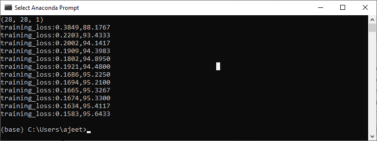

Step 13:

Now, we will append the accuracy for the entire epoch into our correct_history list, and for better visualization, we will plot both epoch loss and accuracy as

Epoch Loss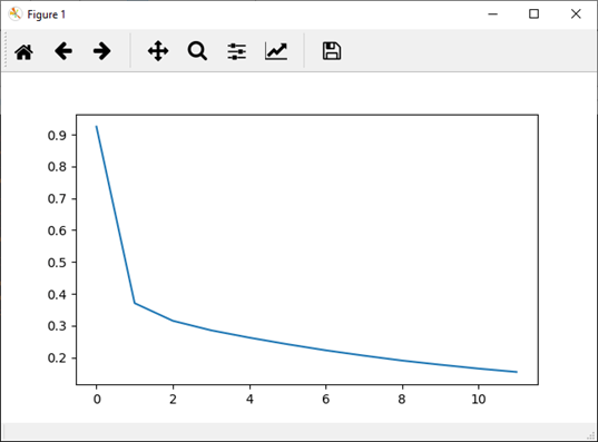

Epoch accuracy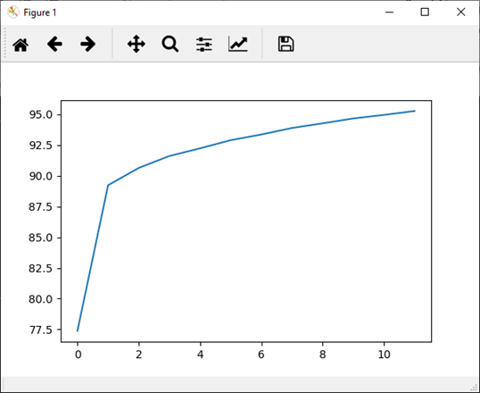

Complete Code