Arrow keys in Excel

Data in Excel can be represented in the form of charts and graphs. The users can communicate data using charts and graphs. Adding the arrow mark in the graph or chart is suggested to establish the relationship between the data. The methods to insert arrow marks in the Excel worksheet are explained in this tutorial.

Why insert an arrow mark in Excel?

Some of the reasons why to insert arrow mark in Excel is explained here as follows:

• The arrow mark in the data helps to indicate the trend and direction of the data. Each arrow mark represents a respective meaning, as the upward arrow indicates positive growth, and the downward arrow implies negative growth.
• Arrow can be used in conditional formatting rules. For example, the user can set the conditional formatting rule to indicate the green arrow mark to the value more significant than a particular value in the data.
• In the flowchart or graphical representations, the arrow mark represents the relationship between the data.
• The arrow mark is used in data validation, which displays the arrow mark in the drop-down list. The arrow mark present in the list helps to choose the option quickly and easily.
• The arrow keys added in presentations and reports highlight the critical points and display the data in an organized form.

Points to Remember before inserting the arrow mark

Some of the issues to be remembered before inserting the arrow mark.

Decide the purpose

The user can decide the purpose of the data before choosing the arrow mark. The number of arrow marks can be fixed based on the content, and the required destination is selected. By determining the purpose, the user can easily place the spot appropriately.

Direction of the arrow

The user can decide the direction of the arrow mark before inserting it. The focus of the arrow mark determines the relationship between the data and the continuity of the data, and it draws the user's attention.

Colour of the data

The user can customize the arrow mark using the Excel feature. The arrow mark's look can be attractive by choosing the desired colour. Another option is to make the arrow mark bold, which draws the user's attention.

Methods to insert the arrow keys in Excel

The various techniques to insert the arrow keys in Excel are explained here.

Steps to insert arrow as a symbol

The user can insert the arrow mark as a symbol. Select the cell where the arrow mark needs to be inserted. In this example, the cell A1 is selected.

Now click Insert> Symbol from the Text group in the Ribbon tab.

The Symbol dialog box will appear. In that, choose the required arrow mark, which needs to be inserted in cell A1.

Click the Cancel option to exit the symbol dialogue box.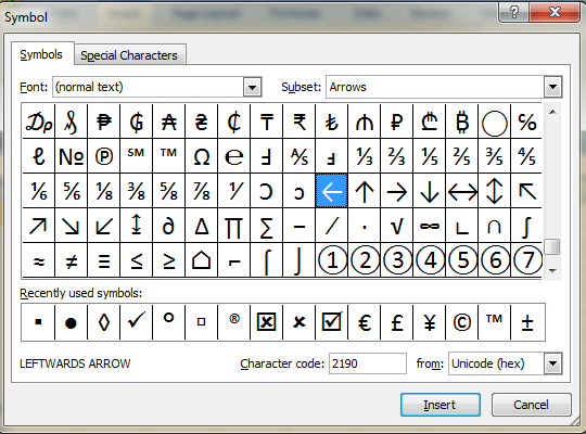

The left arrow mark, which is displayed in cell A1, is chosen.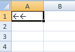

Steps to insert arrow as a shape

The user can insert the arrow mark as a shape.

Select the cell where the arrow mark needs to be inserted. In this example, the cell A1 is selected.

Now click the option Insert> Shapes from the Illustration group in the Ribbon tab.

Choose the arrow mark present in the Line group and drag it into the particular cell.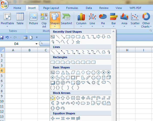

The correct arrow mark, which is displayed in cell A1, is chosen.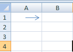

Steps to insert arrow mark with a drawing tool

The user can insert the arrow mark with a drawing tool. The user can create a custom arrow with unique designs using a drawing tool.

The steps to be followed to insert the arrow mark with a drawing tool are as follows:

The draw tab should be added in the top banner to insert the arrow using the drawing tool. Click the File tab

In the drop-down menu list, select "Options."

Choose the option "Customize Ribbon".

Click the box present next to "Draw".

By pressing the "OK" button, the draw tab is added to the top banner.

In the draw tab, the pen is used to create the arrow

Click on the lasso icon and choose the option "Shape".

Select the option "Ink to Shape" present in the draw tab.

Steps to insert arrow mark into a column chart

The user can insert the arrow mark into a column chart. Using a column chart, the user can convert the bar into arrows. The arrow mark in the column chart indicates the relationship between the data and implies the growth or decline based on the time.

The steps to be followed to insert the arrow mark into a column chart are as follows:

Click Insert>Shapes option from the Illustration group

Choose the desired arrow mark present in the "Block arrow" section. In this example, the upward arrow mark is selected.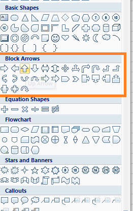

After clicking, move the cursor out of the dialogue box option. Click the required cell where the arrow mark is to be displayed.

In the example, the arrow mark is displayed in cell A1, and it is cropped based on the choice of preference, shown in A1 to A5.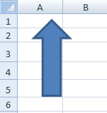

Note:

In the image, the arrow mark is inserted in the worksheet. To display the arrow mark inside the chart,

Click the required arrow mark and click the keyboard shortcut key Ctrl+C to copy the arrow mark.

Click the keyboard shortcut Ctrl+V to paste the arrow mark in the chart.

Steps to insert arrow mark into a line chart

The user can insert the arrow mark into a line chart. Using a line chart, the arrow mark is used to show the trends in the data set.

The steps to be followed to insert the arrow mark into a line chart are as follows:

Enter the raw data in a cell range A1:B10 and insert the line chart for the data as follows: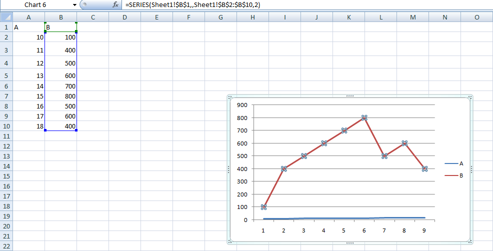

Right-click the line; there are several options. In that, choose the option "Format Data Series".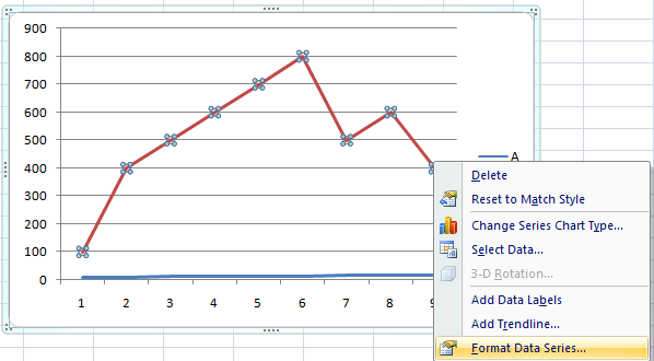

The Format Data Series dialog box will appear. In that, choose the option called "Line Style".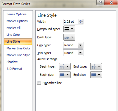

Select the desired arrow from the Arrow Settings.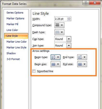

The arrow mark will be inserted in the chart, as shown in the image.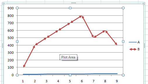

Steps to insert curved arrow mark in the data

The user can insert the curved arrow mark in the data. The curved data mark is used to establish the relationship between the data

The steps to be followed to insert the curved arrow mark in the worksheet are as follows:

Click Insert>Shapes option from the Illustration group

Choose the desired curved arrow mark in the "Block arrow" section. In this example, the curved arrow connector is selected.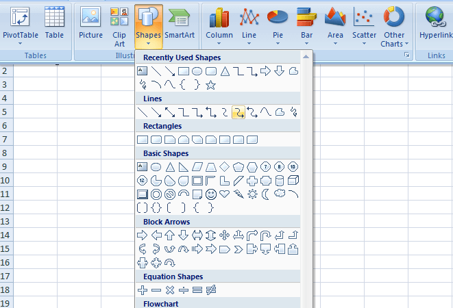

Place and click the cursor where the arrow mark needs to be displayed. In this example, the cursor is placed in cell A1.

Draw the arrow using the mouse for the required arrow position in the worksheet.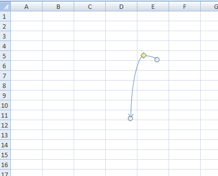

Summary

Arrow keys play a vital role in establishing the relationship between the data. This tutorial discusses the various methods to insert the arrow mark. The user can choose the appropriate way to insert an arrow mark based on the user's requirement.