How to Create Mark Sheets in Excel?

What Is Excel Marksheet Format?

An Excel worksheet is built into an Excel workbook to keep track of cumulative data for analysis now and in the future. It assists us with tracking the output of students in a college or university, staff members in a business, etc.

An Excel Marksheet format represents an automatic Marksheet that provides the necessary information when we add new data or update the current data.

Important points:

• Calculating the students' results is the purpose of the Excel marksheet.
• With the help of formulas and the Marksheet format, results are calculated, such as the total, average, or count of students who meet certain requirements, etc., using Excel functions like IF, SUM, AN AVERAGE, COUNTIF, ROUND, etc.
• We can use conditional functions like IF() and COUNTIF() to give an alternate output rather than the default "True" or "False," as we observed in the examples where the output was displayed as Passing or Failing, Improved or Distinction, etc.

How Do I Create a Marksheet in Excel?

We can create a marksheet using Excel format using the methods listed below.

1. SUM function.
   
   1. Comma Function
2. Colon Method
3. AVERAGE Function
4. ROUND is a function.
5. IF statement.
6. COUNTIF function

1. SUM Function

It adds the values of the selected numeric cells and returns the total. It has the following syntax:

a. SUM function - Comma Method - Using commas, we separate the cell values in the Formula in this method.

The following example shows the marks of a class's subjects, and the total marks will be determined through the Microsoft Excel SUM Function Comma Method.

The following are the steps to evaluating the results with the Excel SUM Function Comma Method:

Step 1: Select cell F2.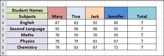

Step 2: In cell F2, we will enter the Formula for the Excel SUM Formula.

• Enter 'number1' as B4, i.e. the sum of all the numbers in cell B4.
• Enter 'number2' as C4, i.e. the sum of all the numbers in cell C4.
• Enter 'number3' as D4, i.e. the sum of all the numbers in cell D4.
• Enter 'number4' as E4, i.e. the sum of all the numbers in cell E4.

As a result, the complete Formula in cell F4 is =SUM(B4, C4,D4,E4).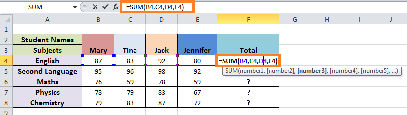

Step 3: Press the "Enter" key. The resulting number is "342" in the picture below.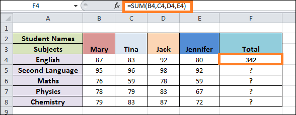

Step 3: Drag the given Formula from cell F4 to F8 by applying the fill handle in Excel. The result is displayed below.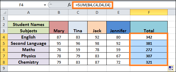

2. Colon Method (Shift Method) - SUM Function The cell values can be entered by choosing the ranges or dragging the cursor by the required cells.

Using the same example as before, we will use the Microsoft Excel SUM Function Colon Method for calculating the marks for the subjects of the students in a class as well as the total marks.

The following are the steps for evaluating the results with the Microsoft Excel SUM Function Colon Method:

Step 1: Select cell F4.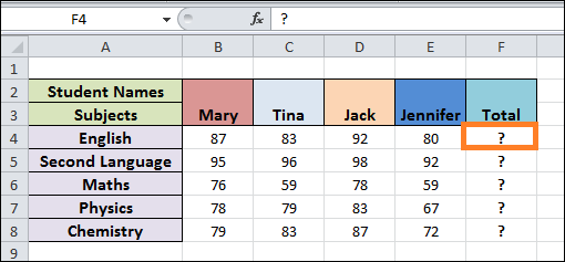

Step 2: In cell F4, enter the following Formula into Excel: SUM Formula =SUM(B4:E4).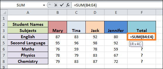

Step 3: Click the "Enter" button. The resulting number is "342" in the picture below.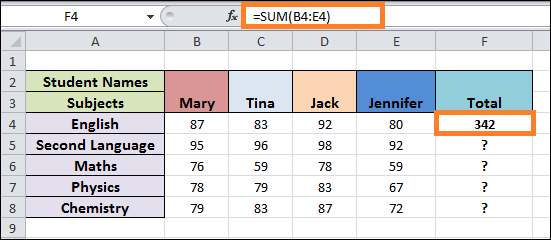

Step 4: Using the fill handle, drag the given Formula across cell F4 to F8. The results are shown below.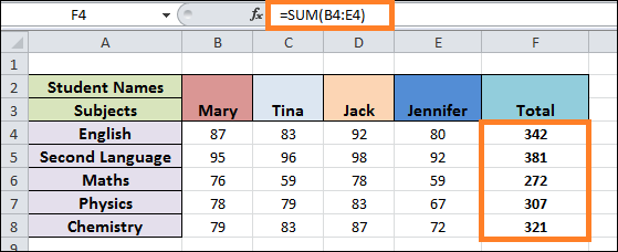

Output Observation: As a result, both the Comma Method & the Colon Method of the SUM function produce the same result.

2. THE AVERAGE Function

It provides the average of all the numerical values you've chosen. Numbers, percentages, and time can all be used as values. The function computes the sum of all the values and divides it into the count for the list's values.

For example, the data below represents the subject marks of students in a class, and we will compute the average marks with the MS Excel AVERAGE Function.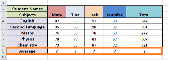

The following are the steps to take for analyzing the values with the AVERAGE Function:

Step 1: In cell B9, type the Formula =AVERAGE(B4:B8).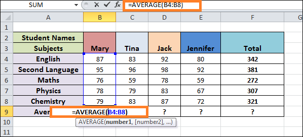

Step 2: Hit the "Enter" button. As shown in the image below, the result is "83".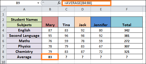

Step 3: Drag the given Formula between cells B9 and F9 using the fill handle. The results are shown below.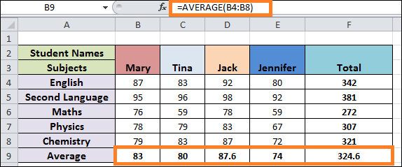

3. ROUND FUNCTION

It rounds up numerical data based on the total number of numbers allocated to round each value.

ROUND operations Arguments Explanation

• It is a number that we intend to round upward or downward. It is a required argument.
• The amount of digits to round up is specified by num_digits. It is a required argument.

The grade and average for each subject for a class of students are shown in the example below. We will use the Microsoft Excel ROUND Function to get the average result's round value.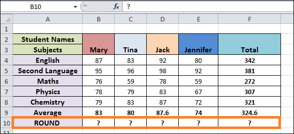

Use the Microsoft Excel ROUND Function to assess the values by following these steps:

Step 1: FirSelectll B10 and type =ROUND(B9,0) into the Formula.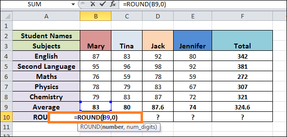

Step 2: Press the "Enter" key. According to the image below, the outcome is "83."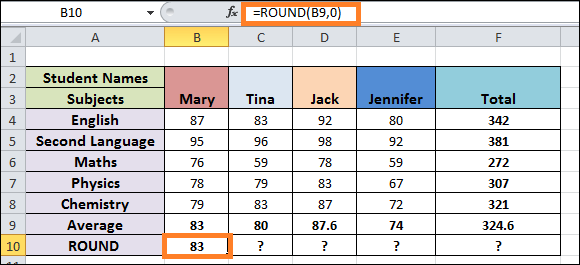

Step 3: Use the fill handle to drag the Formula across cell B10 to cell F10. Below is an example of the output.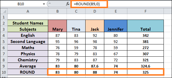

4. IF Function

The output is indicated as true or false after testing the logical conditions. With the help of mathematical operators, it also runs analytical tests on the supplied data. Arguments can produce results other than true or false.

The results of two subjects for a class of students are shown in the following example. Applying the Excel IF Function, we will determine whether the students pass or fail.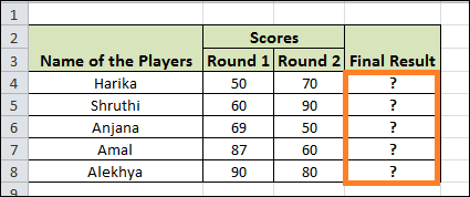

The following are the steps for evaluating the values with the Excel IF Function:

Step 1: First, choose cell D4 and type =IF(AND(B4>=50, C4>=75), "PASS," "FAIL").

Note: The condition values found in cells B4 & C4 constitute the "logical test" value, which is B4>=50 AND C4>=75.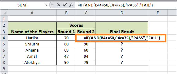

Step 2: Hit the "Enter" keyboard. The image below shows "PASS" as the outcome.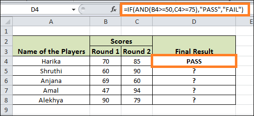

Step 3: Drag the Formula from cell D4 to cell D8 using the fill handle. The result is displayed below.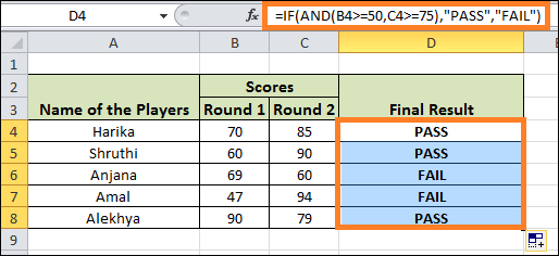

5. COUNTIF Function

It counts every cell whose value falls within the range the conditions give.

COUNTIF Functions arguments explanations:

• Range: The criteria argument is used to apply to this range. It is an essential argument.
• Criteria: It is a requirement on the argument's range of values. It is an essential argument.

The yearly results for each subject for a class's students are shown in the example below. We will use the Microsoft Excel COUNTIF Function to find students with scores above 75.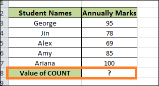

The following are the steps to use the Microsoft Excel COUNTIF Function to evaluate the values:

Step 1: Choose cell B7 and type =COUNTIF(B3:B7,">75"), meaning that B3:B7 is the "range" value and ">75" is the "criteria" value.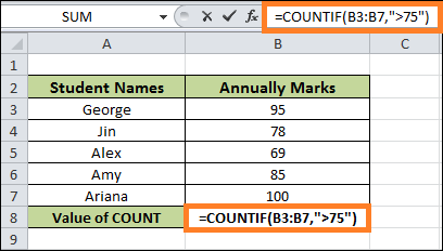

Step 2: Click or tap "Enter." As a result, there are four cells (cells B3, B4, B6 and B7) in the range of cells B3 to B7, or "4" in total.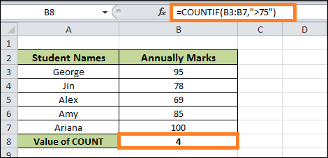

Key Points To Remember

• We will receive the "#NAME?" error if any of the formulas are not written in the proper syntax.
• As with the IF COUNTIF function examples, double quotes("") should be used when entering any content in the function, just as we did when writing "Pass," "Fail," etc.
• The formulas find the total of the remaining numeric values, regardless of the functions used, if the dataset contains non-numerical values in the Marksheet.