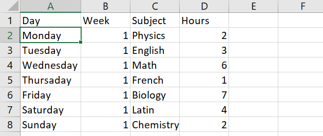
How to Color Alternate Rows in Excel

A simple and efficient method for improving the comprehensibility of your Excel spreadsheets and facilitating a quicker knowledge of the information is to colour alternate rows in Excel. This method involves applying various background colours to each row to improve visual clarity, which can be especially useful when reading and interpreting large datasets.

You'll utilise conditional formatting in Excel to apply rules depending on particular criteria to accomplish this formatting. This systematic process is part of choosing the appropriate range, going to the "Home" tab, using conditional formatting choices, and configuring a formula to identify the formatting pattern.

Basic Steps to Alternate Row Colors in Excel:

One easy yet powerful approach to make your data easier to read in Excel is to color-codes your rows. The following are the fundamental procedures for using conditional formatting to achieve alternating row colours:

1. Open your Excel Spreadsheet:

Open the spreadsheet with the data you wish to format in Excel.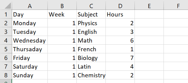

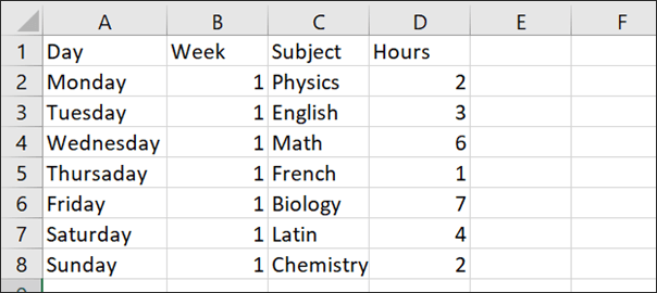
2. Select the Range:

Click and drag to choose the range of cells you wish to format with alternative row colours. Ensure that you include the complete dataset.

3. Navigate to the "Home" Tab:

Select the "Home" tab from the Excel ribbon that appears at the highest point of the screen.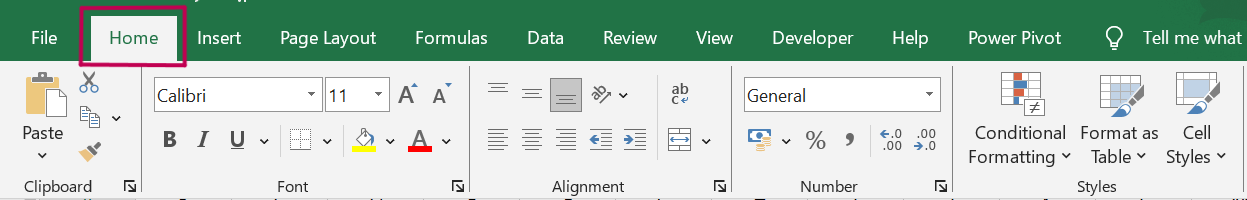

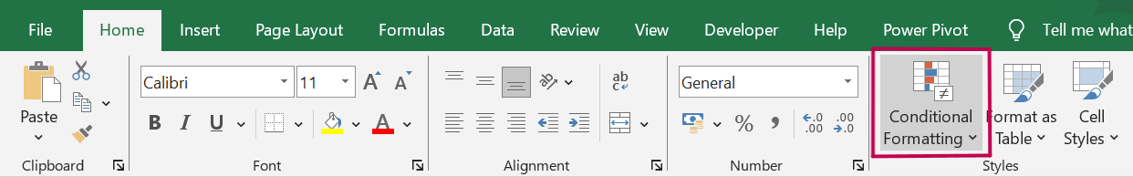
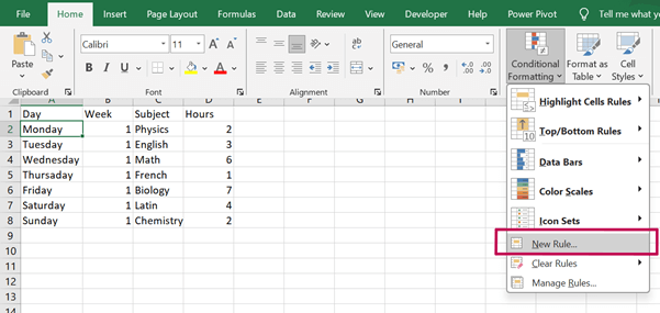
4. Access Conditional Formatting:

Look for the "Conditional Formatting" toolbar alternative. It's generally located inside the "Home" tab's "Styles" or "Format" institution.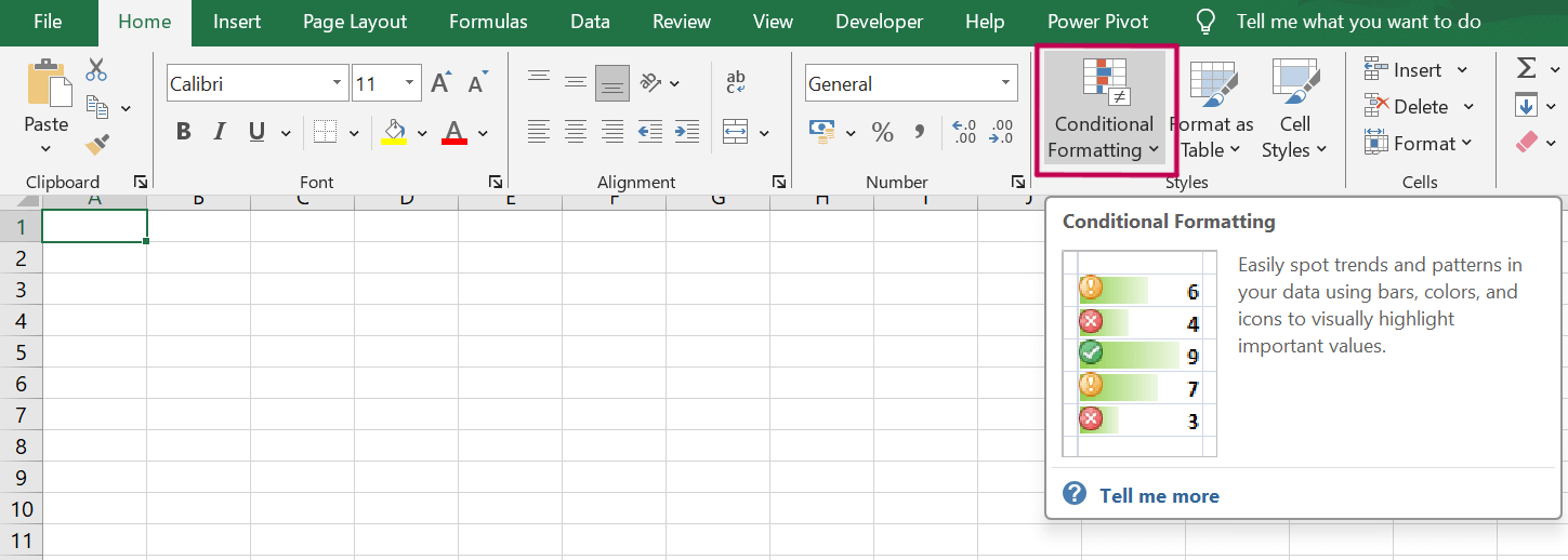

5. Choose "New Rule":

Choose "New Rule" from the drop-down box underneath "Conditional Formatting." The "New Format Rule" speak container seems as a result.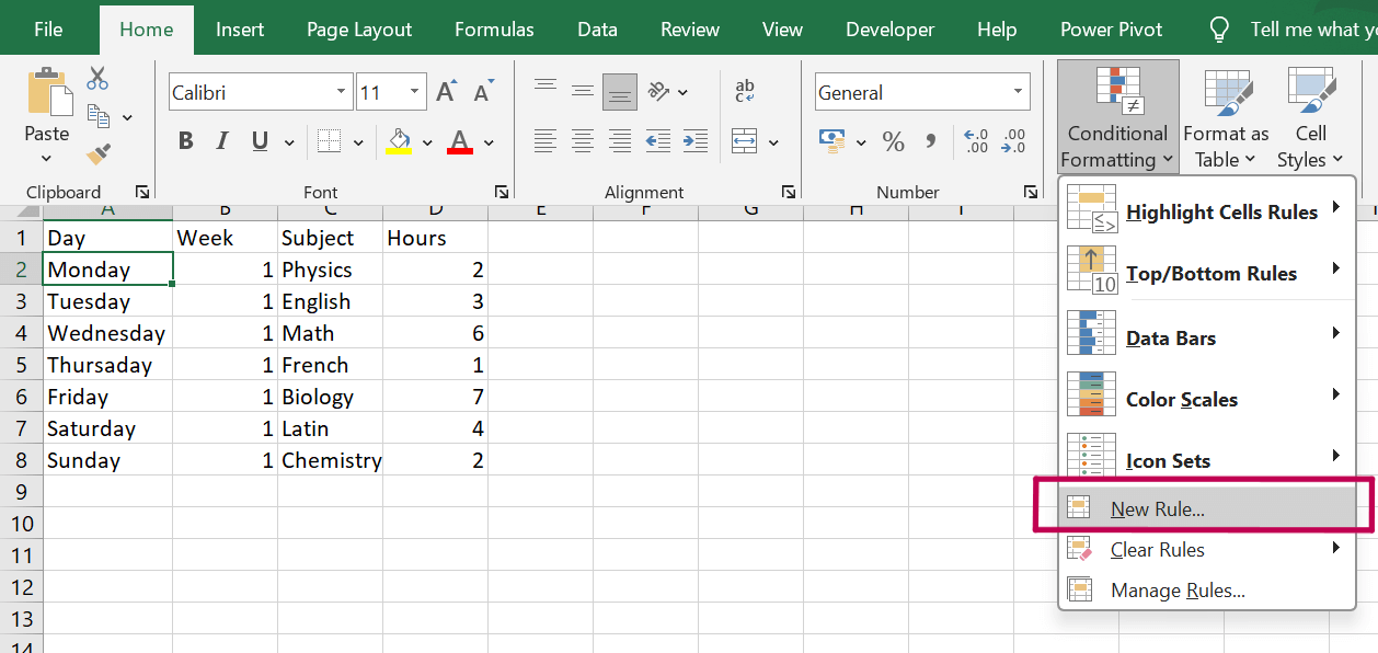

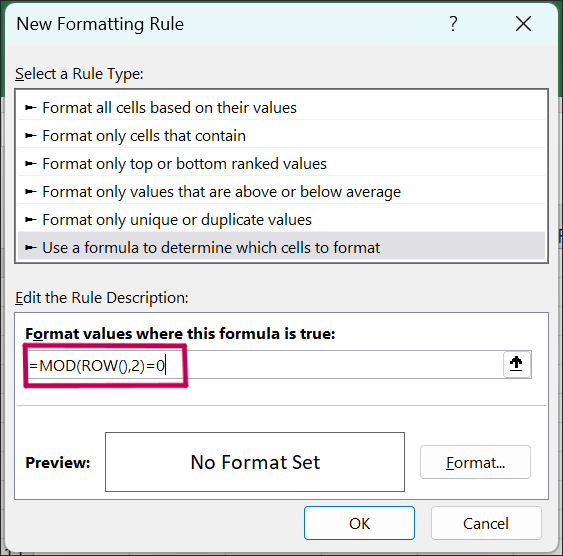
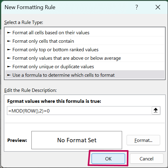
6. Select "Use a Formula to Determine Which Cells to Format":

To format cells, use a formulation. This choice can be located in the "Select the Rule Type" window.

7. Enter the Formula:

In the certain discipline, kind the following method:

=MOD(ROW(),2)=zero

This system shows exchange rows by using figuring out if the row integer is even.

8. Set the Format:

Select "Format" through clicking on it. Choose the heritage shade for the even rows by using choosing the "Fill" tab in the "Format Cells" talk box. Press "OK" to affirm.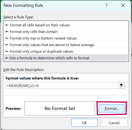

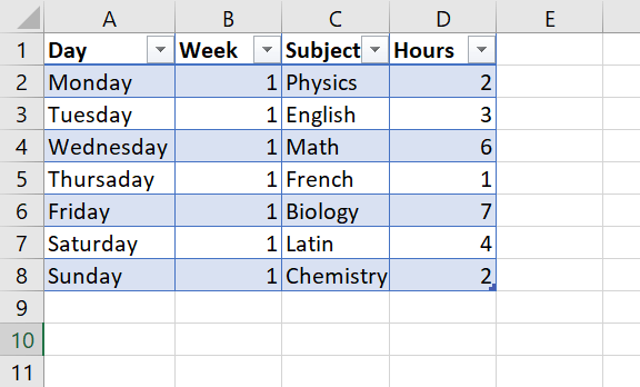
9. Apply the Format:

Click "OK" over again within the "New Format Rule" window to use the exchange row shades to your preferred variety.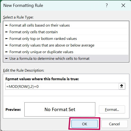

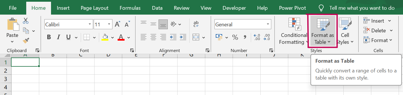
How to Use Conditional Formatting to Alternate Row Colors in Excel:

Use conditional formatting to get the same effect without using pre-set table styles or if you want greater influence over the colour scheme. How to do it is as follows:

• Choose the cells to which you wish to apply formatting. Then, select Home > Conditional Formatting >. New Guidelines
  
• Choose "Use a formula to figure out which cells to format."
• Type in "=MOD(ROW(),2)=0" as the formula.
  
• Select the format you want for the cells.
• Select OK.
  

Depending on your preferences, you can modify the formula to alter the row number or the cell format.

Cells that match specific criteria can also be highlighted using conditional formatting. For instance, you may apply conditional formatting to highlight all the cells that have the term "Total" or any other value. To apply the formatting: Pick the cells you wish to format, then choose the Home tab > Conditional Formatting > New Rule option. Choose "Use a formula for figuring out which cells to format" and type in the formula "=SEARCH("Total", A1)>0" (assumed to be in column A). Select the format you want for the data fields and press OK.

Using Formulas to Alternate Row Colors in Excel:

With a fundamental formulation and Excel's conditional formatting function, you could utilise formulas to trade the shade of rows. How to do it's far as follows:

• Choose the cell range to which you wish to apply the formatting.
• Navigate to the "Home" tab and pick "New Rule" under "Conditional Formatting."
  
• Select "To decide which cells to format, use a formula.Put "=MOD(ROW(),2)=0" for even values and "=MOD(ROW(),2)=1" for odd values into the formula.
  
• After selecting the formatting alternatives you need, click OK.
  

It's vital to consider that you should not tough-code the coloration values into Excel formulation in case you want to use them to change the row colours. Instead, use named degrees or cellular references to make it simpler to replace the colours later. Additionally, this may make using the same coloration scheme less complicated throughout several workbooks or worksheets.

Understanding the Benefits of Alternating Row Colors in Excel:

Excel's exchange row shade characteristic offers various advantages. First of all, dividing information blocks and preventing confusion among diverse rows improves readability. Second, it enables the short identification of errors or anomalous developments in the statistics, enhancing your analysis's efficacy. Finally, it enhances the arrival of your Excel worksheet and offers it a sophisticated look.

One gain of the use of alternating row colorings in Excel is that it helps statistics comparisons between rows. You can swiftly decide which rows consist of same records and which range by using assigning wonderful colorations to every row. This can be pretty beneficial when coping with massive datasets or trying to spot patterns and developments in the facts.

When using Excel for a long period, rotating row colours can also aid in lessening eye strain and tiredness. Concentrating on particular columns and rows can be simpler without being overcome by the quantity of data displayed on the screen if the material is divided into more manageable portions. In addition to decreasing errors and increasing productivity, this can enhance the general enjoyment of using Excel.

How to Apply Alternating Row Color to Multiple Sheets in Excel:

The Format Painting tool in Excel can apply alternate row colours to numerous pages. How to do it is as follows:

• Choose the cells that have already been formatted with the alternate row colours.
• Select the Home tab. Painter of Formats
  
• Select the worksheet you wish to format by clicking on its sheet tab.
  
• Choose the cell range to which you wish to apply the formatting.
  
• The chosen cells will receive the alternate row colours.
  

For each sheet you wish to format, comply with these steps over again. Using this approach, you may without problems follow equal formatting to numerous sheets without requiring the layout and implementation of a theme.

Customizing the Color Scheme When Alternating Rows in Excel:

When switching rows, Excel offers many possibilities for customizing the color scheme. With the "Conditional Formatting" device, you may design your color scheme or pick from various pre-set designs. The following are some factors to bear in mind:

• Select complementary colours that do not overpower each other.
• Please chorus from the usage of too many shiny or putting hues because they'll be overpowering.
• Try to hold the same coloration palette for all worksheets and tables.

Ensuring the colors you pick out are readable with the aid of manner of all clients, mainly humans with colour imaginative and prescient impairments, is important to not forget about even as enhancing the color scheme in Excel. To make certain that the data and foreground shades adhere to accessibility hints, you may make use of internet tools to diploma their evaluation ratio.

Furthermore, you may look at several color schemes in keeping with your spreadsheet's statistics via conditional formatting. You can use an inexperienced coloration scheme for excellent values and a purple colour scheme for terrible ones. This would possibly help you notice styles and trends for your data faster.

Troubleshooting Common Issues When Alternating Rows Colors in Excel:

When changing row colourings in Excel, you may run into issues even if you entire all the commands exactly. The following are some everyday issues and their fixes:

• The colorings do not properly trade: Verify which you have selected the entire desk and that the row equation is accurate.
• As quick as you filter or kind records, the colours vanish. After deciding on or filtering, use the "Format as Table" and "Conditional Formatting" options, or adjust the calculations to consist of columns.
• Depending on the device, the colors appear warped or in some other way: Verify that the colour scheme and Excel version you're using are the identical.

Conclusion:

To sum up, there are numerous strategies to color alternating rows in Excel over numerous sheets: you can use formulation and Excel Tables or Conditional Formatting. Excel Tables provide an easy answer. Excel will mechanically follow alternating row hues even as you create a desk and choose a fashion. By copying and pasting, this technique makes replication throughout several sheets simple.

However, extra flexibility is offered with Conditional Formatting with Formulas. You can specify a component to select which rows to layout the use of the MOD characteristic interior a conditional formatting rule. This technique creates a rule based totally on row values and then applies it to an appropriate variety. Similarly, you can replica and paste the formatting to greater sheets.

Select the method that high-quality meets your wishes and alternatives. Excel Tables are effective and smooth to use, however Conditional Formatting offers you extra customization alternatives. Whichever way you pick out, via the usage of specific colorings for each row, you can improve the visible readability of your information and make it smooth to study and understand.