Subtotal with Countif Function in Microsoft Excel

Microsoft Excel stands as a cornerstone tool that is quite responsible for the purpose of offering versatile functions in order to manipulate the dataset and also to analyze it. Among all these, the respective "Subtotal function" and "Countif functions" emerge as indispensable allies, responsible for empowering the users to perform various intricate calculations swiftly and accurately.

However, the "Subtotal function" in Microsoft Excel primarily serves as the powerful aggregator, which enables the respective users to easily compute out the various summary statistics, which are none other than sum, average, count, and many more that lie within specified subsets of the data effectively. Coupled with the "Countif function," which tallies out the occurrences of the specified criteria within a given range of the data, Microsoft Excel users gain enhanced control over their data analysis endeavors, and this introduction sets out the stage for exploring the synergistic relationship that mainly exists between the Subtotal and Countif functions, and also understanding their basic definition with syntax and day to day life example then elucidating how their combined prowess facilitates the streamlined data analysis processes. Through practical examples and insights, this tutorial aims to equip users with the knowledge and the proficiency to harness all these functions effectively, unlocking deeper insights and driving informed decision-making in Excel-based data analysis workflows, respectively.

What is a SUBTOTAL function in Microsoft Excel?

The respective "SUBTOTAL function" in Microsoft Excel is usually considered a versatile tool that is efficiently designed for the purpose of performing aggregate calculations on the data ranges. And unlike the traditional functions such as SUM or AVERAGE, SUBTOTAL mainly adapts to filter out the data, and computing out the results that are based solely on the visible cells within the specified range respectively. This feature is very much invaluable for scenarios where the subsets of the data need analysis without interference from the filtered-out or hidden cells. By just incorporating the various function numbers, like as SUM, AVERAGE, COUNT, and others, SUBTOTAL offers flexibility in the generation of the different types of subtotals or totals within the given datasets. Whether managing financial records, inventory lists, or sales data, SUBTOTAL usually enhances efficiency by just automating the calculations and ensuring accuracy across a huge number of datasets. Its ability to seamlessly adjust calculations based on changes in data visibility or filtering simplifies complex data analysis tasks. Moreover, the SUBTOTAL function is particularly beneficial for generating the subtotals within the grouped data, thus providing a streamlined approach to the analysis of the data without the need for manual adjustments or to separate the calculations. In essence, the SUBTOTAL function empowers Excel users to easily perform the comprehensive analysis of the data efficiently, making it an indispensable tool for professionals across various industries.

Syntax of the SUBTOTAL function in Microsoft Excel

The syntax that can be efficiently used for the "SUBTOTAL function" in Microsoft Excel sheet is as depicted below respectively: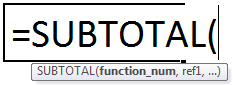

More often, the SUBTOTAL function primarily accepts the following arguments, which are discussed below:

• Function_num: This number is mainly responsible for determining which arithmetic operation (function) will be performed by the SUBTOTAL function. Despite this, the "function_num" argument can easily take any value ranging from 1 to 11 or 101 to 111, respectively.
• Ref1: This is the range of the cells on which the arithmetic operation needs to be performed. Despite this, it can be easily supplied as a reference or as a named range, respectively.
• Ref2: This argument in the SUBTOTAL function is considered the second range of cells on which the arithmetic operation must be performed. It could also be entered as a reference range or as a named range. The arguments "function_num" and "ref1" are mandatory, while "ref2" is optional. The SUBTOTAL function returns a numeric output.

Important Note: It should be noted that, the "function_num" argument is always entered as a numeric value and not as the string or character respectively.

How to open the SUBTOTAL Function in Microsoft Excel?

Now, for the purpose of opening out the "SUBTOTAL Excel function" in Microsoft Excel, we are required to enter the "=SUBTOTAL" in the required cell that the arguments of the function have followed. In alternate to this, the respective SUBTOTAL function can also be opened from the Formulas tab of Microsoft Excel. The steps for the same are listed as follows:

Step 1: First, we must select the cell in which the" SUBTOTAL formula" is to be entered.

Step 2: Now, from the Formulas tab, we must need to click on the dropdown menu of the "Math & Trig" option. After that need to select the "SUBTOTAL", as clearly depicted in the following image: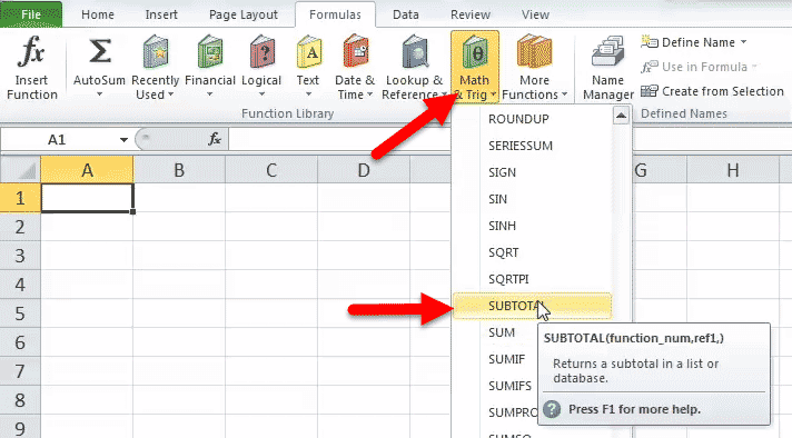

Step 3: Often, just after applying the above step, we will be encountered with the "function arguments" dialog box, as it was clearly depicted in the following image. Here in this dialogue box, we are required to enter the values for the arguments "function_num" and "ref1," respectively. Once the cursor is placed inside the "ref 1" box, the "ref2" box appears just below it respectively.

After this, we need to click on the "OK" button to proceed further with the outcome. The output of the SUBTOTAL function will be displayed in the cell selected in Step 1, respectively.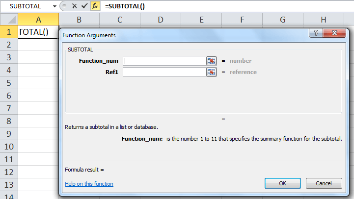

What are the three reasons to make use of the SUBTOTAL function in Microsoft Excel?

The three important reasons to effectively make use of the SUBTOTAL Function in Microsoft Excel are as follows:

1. Calculation of the respective values in the filtered rows.

It is well known that the SUBTOTAL function in Excel usually ignores the values available in the filtered-out rows. With this, one can also create a dynamic data summary where the subtotal values are recalculated automatically in accordance with the filter.

• For example, Here we will be considering a case where we will be filtering out the table in order to show the sales only for the East region. Also, the Subtotal formula will automatically be adjusted so that all other regions are removed from the total:

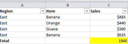
2. In the Excel sheet calculate only visible cells.

As we all know, the respective "Subtotal formulas" with function_num 101 to 111 basically ignore the entire hidden cell. So, when we use Microsoft Excel's Hide feature to remove irrelevant data from the view, we are required to use function numbers ranging from 101 to 111 to exclude values in the hidden rows from the subtotals, respectively.

3. Ignoring values in the nested Subtotal formulas.

Let us assume the range that has been effectively supplied to our respective Microsoft Excel Subtotal formula contains any other Subtotal formulas. In that case, all those nested subtotals will be ignored, so the same numbers will only be calculated once.

As in the screenshot below, the Grand Average formula SUBTOTAL (1, C2:C10) usually ignores the results of the Subtotal formulas in the given cells, C3 and C10, as if we used an Average formula with the 2 separate ranges AVERAGE (C2:C5, C7:C9).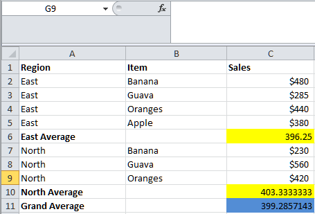

# Example 1: Making use of the SUBTOTAL function in Microsoft Excel

Step 1: Firstly, we need to construct a small table that contains data from the different categories, as mentioned below.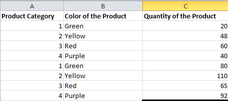

Step 2: In this step, we need to observe the above table. By observing, we noticed that we have a product category, color category, and quantity of the product. After that, we must apply the "SUBTOTAL formula" as mentioned below with function number 9.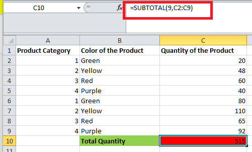

Step 3: After that, we are required to apply this formula and the result depicted below, respectively.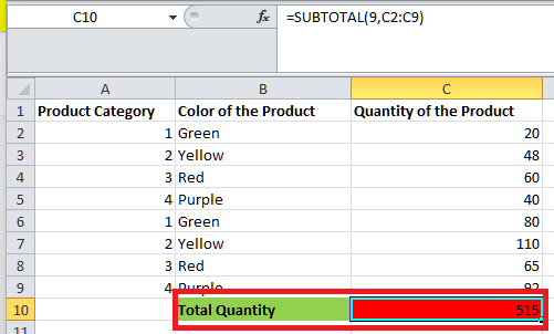

Step 4: In this step, we are required to apply the "SUBTOTAL formula," as mentioned below, with the function number 109.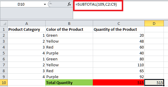

Step 5: Now, we must apply the SUBTOTAL Formula, and the result is as depicted below.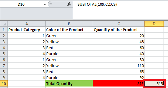

Step 6: In this step, we have used function numbers 9 and 109 in the formula to perform SUM in two columns. C2:C9 is the range of the data on which we are actually performing the calculations, respectively. The total sum is 515 for both formulas. Now, hide some of the rows and then observe the results for both formulas.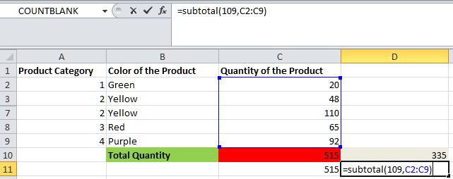

Step 7: And now in this step, just after applying the "SUBTOTAL Formula," the result is usually depicted below respectively: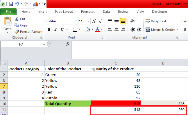

Despite all this, the respective rows from rows 50 to 60 are hidden; hence, the results of function number 109 have changed to 260. This is because it does not consider the manually hidden data, whereas function number 9 remains the same, meaning it will consider the data even though we hide it manually.

Step 8: Now, we will apply a filter to the data and then filter only one color; in this example, we have considered the "Yellow Color."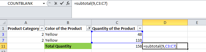

Step 9: Just after applying the "SUBTOTAL Formula," the result is as depicted below.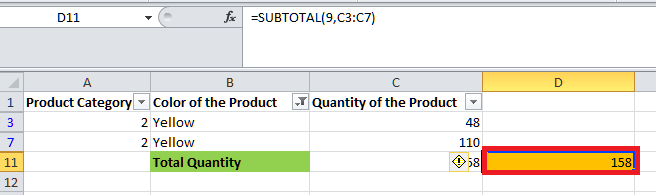

And then, we need to apply the SUBTOTAL Formula as mentioned below with Function Number 109.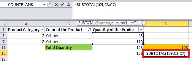

Step 10: And now after applying the "SUBTOTAL Formula," the result is as shown below.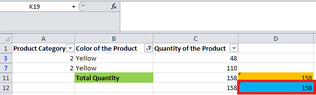

Now if we observe the screenshot mentioned above, we can see that both the function numbers did not consider the quantity of the filtered-out data. After we filter out the data and hide rows, both the formulas will give the same results that both the formulas will not consider out the non-visible data.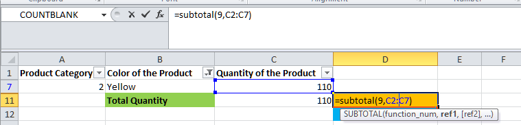

Step 11: After applying the SUBTOTAL Formula, the result is as shown below.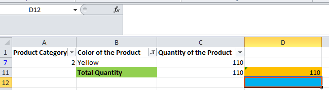

Step 12: Apply the SUBTOTAL Formula as below with Function Number 109.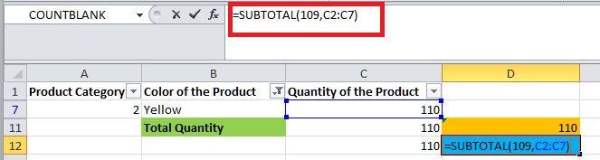

Step 13: Now, after applying this formula, the result is shown below.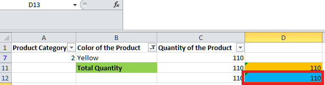

What is meant by the term COUNTIF function in Microsoft Excel?

The respective COUNTIF function in Microsoft Excel is a powerful tool that can be used for the purpose of counting out the number of cells within a specified range that usually meets a given condition or criteria. Its primary purpose is to provide a quick as well as efficient way to tally out the data, which are based upon some of the specific parameters, thus enabling the users to analyze as well as to manipulate the large sets of information with ease.

1. The COUNTIF Excel Function is mainly used for the purpose of counting the cells with the numeric as well as the alphabetic values in a given range or array, which is based upon the test condition as well as effectively returns the accurate result.
2. When making use of this function, numerous criteria or test conditions can be easily specified in a single dataset.
3. The "Formulas" > "Function Library" > "More Functions" > "Statistical" menu item usually provides access to the function.
4. One can double-click on the COUNTIF function from Excel's list of the suggested functions by typing =C and then selecting it from the list or by just typing =COUNTIF (in a cell).

The syntax for the COUNTIF function in Microsoft Excel

The syntax of the COUNTIF function is quite straightforward: it mainly consists of two main components: the range as well as the criteria. The "range" refers to the group of cells that we actually want to evaluate, while the "criteria" establishes the condition that must be met for a cell to be included in the count as well. This condition is capable of taking out the various forms, which will include the following ones: numerical values, logical expressions, etc.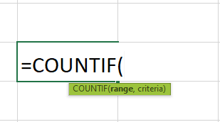

More often, if in case we have a range of cells which are containing some of the numerical data, and here in this, we wish to determine how many of those cells contain values that are greater than the value 30, then it would make use of the COUNTIF function as follows: `=COUNTIF(range, ">30")`. Despite all this, the versatility of the COUNTIF functions primarily makes it an invaluable tool for a wide range of applications, such as financial analysis, statistical reporting, and inventory management. By just providing a simple yet effective means of summarizing data based upon the user-defined criteria, the COUNTIF function mainly empowers the respective users to extract meaningful insights. It helps an individual to make informed decisions.

# Example 2: Use of COUNTIF function with the given values in Microsoft Excel.

For the purpose of utilizing the COUNTIF Function in Microsoft Excel in order to count the occurrences of the specific value within a range of the cells, we need to follow these steps respectively:

Step 1: First, we are required to construct a table that usually depicts a list containing numerical values in cells B2:B7. We are required to count the given range of cells for the values that primarily match the number "43," respectively.

Step 2: And now in this step, we are required to apply the "COUNTIF function" to the given range of the cells, and the formula is stated as follows:

"=COUNTIF (B2:B7, 43)." Here, the respective condition is applied to the formula is the number "43".The formula checks the range of cells B2:B7 for the values matching the number "43". The range contains only one such number, which satisfies the condition.

Step 3: Hence, the result is usually returned by the COUNTIF function as "2." The result is displayed in cell B8, respectively.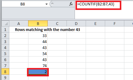

# Example 3: Use of COUTNIF function to count the numbers with a less than the given number.

Now, for the purpose of utilizing the COUNTIF Function in Microsoft Excel in order to count the numbers of the specific value within a range of the cells, we need to follow these steps respectively:

Step 1: A list of the data in the cells B2:B10 is provided in the succeeding table. Count the given range of the cells for the values that are less than "70". After that, the respective COUNTIF function is primarily applied to the given range of the cells, and the formula is stated as follows:

"=COUNTIF (B2:B10,"<70")"

Step 2: Here, the condition applied to the formula is "<70". The COUNTIF formula checks the range of the cells which are matching with the condition, less than 70. There are only four values that are less than 70 in the range. Hence, the result returned by this function is "5". The result is displayed in cell B18 effectively.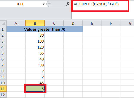

How to easily make use of the SUBTOTAL Function with the COUNTIF Function in Microsoft Excel?

Here, we will focus on how to easily use the SUBTOTAL function with the COUNTIF function to calculate the count of a filtered data set effectively. When we filter out a large set of data only to display certain data values, the function will still count the hidden values and also include them in the calculations.

However, sometimes we want to calculate only the visible rows or the data values of the particular selected data set. If, in case, we want to count the number of cells that meet our given criteria based on the filtered data set. Sometimes, the function will count the entire data set, and to prevent this, we must utilize the SUBTOTAL function, the COUNTIF function, and the SUMPRODUCT function.

#Example: 1 Use of SUBTOTAL with COUNTIF

Let us now take a sample scenario wherein we are required to make use of the SUBTOTAL function with the COUNTIF function in Microsoft Excel. Assuming that we have a set of data that contains a list of the different class scores and also the gender of the selected students, here in this, we actually want to count the number of girls in a specific class. Instead of creating a new data set, we can also opt to filter out the specific class. However, the function is returning the incorrect result. So, we decided to opt to combine the SUBTOTAL and COUNTIF functions to obtain the correct count efficiently.

Now, we will explain the step-by-step process for using the SUBTOTAL with the COUNTIF function in Microsoft Excel. To apply this method to our work, we can follow the steps mentioned below.

Step 1: First, we are required to filter our initial data set. To do this, we will select the entire range and then go to the Data tab. Then, we will select the Filter within the Sort & Filter section, respectively.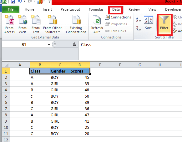

Step 2: After that, we will click on the dropdown arrow made available just beside the Class column. Next, we will check out the box for A since we only want to count out the cells from class A. Lastly, we will press the Apply option.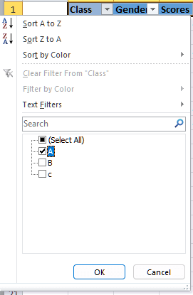

Step 3: Now in this step, after we have filtered out the data set, we can now easily apply the formula. To achieve this, we can input the formula that is none other than: "=SUMPRODUCT (SUBTOTAL (3, OFFSET (C2:C8, ROW (C2:C8)-ROW (C2), 0,1)),-(C2:C8="girl"))," just after entering the formula we are required to press the Enter key from our respective keyboard in order to return the result effectively.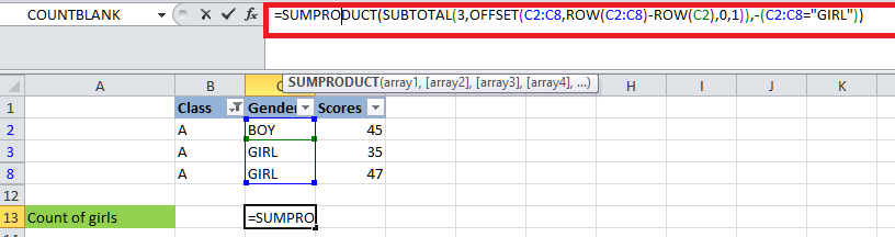

Step 4: And tada! We have successfully used the respective SUBTOTAL with the COUNTIF function in Microsoft Excel.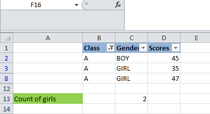

# Example 2: Effective use of the SUBTOTAL Function with the COUNTIF Function

Now in this example, we will be seeing the effective use of the SUBTOTAL Function with COUNTIF Function in Microsoft Excel.

Let us now imagine a spreadsheet with data about basketball players. This particular dataset usually includes the following information: their name, position, and conference. To achieve our desired goal, we will implement the subtotal with the countif function.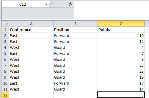

Step 1: First, we need to filter the data to display only the players from the West conference. To achieve this, we must select the entire dataset. After selecting the data, we must navigate to the Data tab, which is available at the top of the Microsoft Excel window, and click on the Filter button. This will effectively add filter arrows to each column header.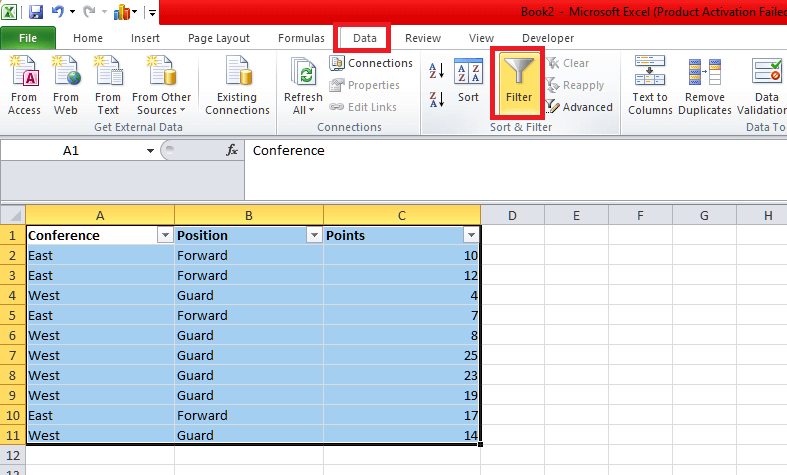

Step 2: Next, we are about to click on the filter arrow available next to the "Conference" column header, and by clicking on it, a dropdown menu will appear with the options to filter by. Make sure only the box next to "West" is checked, and then you need to click on the "OK" option. Our data will instantly update to show only the rows where the conference is West.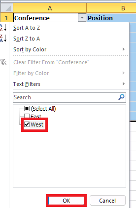

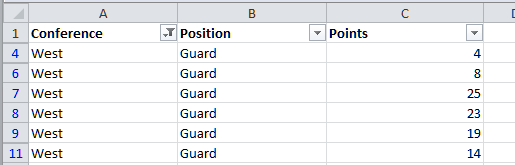
Step 3: More often, to accurately count out the number of the visible rows where the position is "Guard," we will be then making use of the combination of the functions which is none other than the SUBTOTAL and SUMPRODUCT function. Here is the formula which we are going to make use of: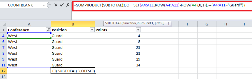

Let's break it down:

1. OFFSET: This function is quite responsible for the purpose of returning a reference to the range that is a specified number of the rows as well as the columns from a starting cell and the starting range.
2. ROW (B2:B11)-ROW (B2): This part of the formula is used to adjust the range to start from the first visible row just after filtering.
3. SUBTOTAL (3): This function calculates the subtotal of a given range using the COUNTA function (3) and considers only visible cells.
4. SUMPRODUCT: Multiplies arrays and then sums the products. In this case, it multiplies the subtotal count by whether each corresponding row is a "Guard."
5. (B2:B11="Guard"): This will convert the Boolean result of (B2:B11="Guard") to 1s and 0s.

Step 4: When we enter this formula into the respective cell, it accurately counts the number of visible rows where the position is "Guard," thus providing us with a reliable count even after applying filters that are none other than 6.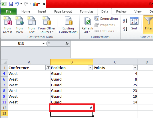

What are the various advantages of using the SUBTOTAL function with the COUNTIF function in Microsoft Excel?

The various advantages of making use of the SUBTOTAL function with the COUNTIF function in Microsoft Excel are as follows:

1. Dynamic Calculation: The respective "Subtotal function" in Microsoft Excel usually allows us to dynamically calculate the subtotals for the filtered data, which is quite useful while combining it with the "Countif function." It means that as we filter or manipulate our data, then the respective subtotal calculations will adjust accordingly, thus providing accurate as well as up-to-date counts that are based upon the filtered criteria effectively.
2. Provides Flexibility in Reporting: By combining the "Subtotal with Countif" function, we can now easily generate customized reports more accurately. Whether we are tracking the number of sales made by a particular salesperson, counting the occurrences of specific items in an inventory, or tallying the responses in a given survey, this effective combination allows for flexible reporting tailored to our specific needs as well.
3. Efficiency: Just making use of the respective "Subtotal with Countif" function can significantly improve efficiency in the data analysis tasks. Rather than manually updating counts or recalculating the totals every time when there are any changes, we can now easily rely upon Microsoft Excel's functions for the purpose of handling these tasks automatically. This will save our time and also reduce the likelihood of errors in our analysis task respectively.
4. Clarity in the Presentation: When presenting the summarized data to others, making use of the "Subtotal with Countif" function will usually ensure clarity as well as transparency to the flow of the data. The subtotal function is mainly responsible for the purpose of providing the subtotal labels that clearly indicate the level of the aggregation, thus making it easier for the readers to easily understand the structure of the data and interpret the counts provided by the Countif function respectively.
5. Helps enhance the understanding of the Data: By breaking down the data into the various subtotals and then applying the Countif to each subtotal, we can easily gain deeper insights into the distribution and patterns within our dataset. This can be particularly valuable for identifying trends, outliers, or areas that primarily require further investigation.
6. Scalability: Whether we are working with a small set of data or a large set of data, the respective "Subtotal function" combined with the Countif scales effectively.

Depicts out the various frequently asked questions about the SUBTOTAL with the COUNTIF function in Microsoft Excel.

The different frequently asked questions about the SUBTOTAL with the COUNTIF function in Microsoft Excel are as follows:

1. List the main purpose of using the SUBTOTAL with the COUNTIF function in Microsoft Excel.

The main purpose is to perform calculations on the filtered dataset. The SUBTOTAL function primarily calculates various functions like SUM, AVERAGE, COUNT, etc., while the COUNTIF function in Microsoft Excel counts out the cells that meet a certain criteria. Combining them allows counting out the filtered data effectively.

2. How can one make use of the SUBTOTAL with the COUNTIF?

We can easily use the SUBTOTAL function with the COUNTIF function by providing the appropriate function number for the COUNTIF as the first argument in the SUBTOTAL function.

3. What are the main function numbers for the COUNTIF with SUBTOTAL?

The function number for the COUNTIF is 109. So, when we use the SUBTOTAL with the COUNTIF, we use 109 as the first argument in the SUBTOTAL function.

4. Can we use other functions with the SUBTOTAL and COUNTIF functions in Microsoft Excel?

Yes, we can also make use of the other functions, such as SUMIF, AVERAGEIF, MAXIF, MINIF, etc., with the SUBTOTAL in a similar way by just providing the appropriate function number.

5. Does SUBTOTAL consider hidden or filtered data?

Yes, of course, the respective SUBTOTAL function ignores the data that is filtered out or hidden, which makes it useful for calculating the results that are based on the filtered data as well.

6. Can we make use of the SUBTOTAL and COUNTIF with dynamic ranges?

Yes, we can easily use dynamic ranges, such as tables or named ranges, with the SUBTOTAL and COUNTIF to automatically adjust calculations as data changes.

7. Are there any limitations to using SUBTOTAL and COUNTIF together?

One limitation is that SUBTOTAL only works with visible cells. If we need to include hidden cells in our calculations, we would need to use other methods or functions.