Spearman rank correlation Calculator Excel

To address the question, "How can the event of load shedding be related to the appearance of a thunderstorm?" we can employ various statistical techniques. To do this, we must first gather a large amount of data from various sources and then analyse it to look for any relationships that might be useful elsewhere. One useful tool for determining whether two occurrences are related to one another or not is the Spearman Correlation. With sufficient examples, this tutorial explains how to compute the Spearman Correlation for two data arrays using Excel.

Why Does the Spearman Correlation Occur?

The Spearman Correlation is a nonparametric counterpart to the Pearson Correlation Coefficient. The linear correlation between two distinct data sets is determined by this number, which is frequently shown by rs or p.

It is possible to ascertain the linear relationship across continuous variables using Pearson's Product Moment Correlation. The Pearson Correlation can be expressed broadly as deviation:

The values ranked already are Rx and Ry. and are the datasets' standard deviations.

Spearman Correlation evaluates the monotonic relationship between values.

The Spearman Coefficient's full form is

This is a significantly altered version of Pearson's formula. Here,
The variables x and y are represented by the letters Rx and Ry.
Mean ranks are denoted by R?(x) and R?(Y).

The Spearman Correlation and Pearson coefficient are rather close; nonetheless, you might need to employ the Spearman Correlation in the event of an outlier.

Applications of the Spearman correlation:

If you have outliers in your data and you know they will affect the outcome. The sensible course of action is to use the Spearman Correlation. This is because outliers affect the Spearman Correlation differently than the Pearson Correlation, due to Spearman's utilization of values' ranks rather than their actual values.
If there is a nonlinear relationship between the data or if they are not properly distributed. The Spearman coefficient outperforms the Pearson coefficient in that case.
If any variables are ordinal, you should use the Spearman Correlation rather than the Pearson coefficient.

The Spearman Correlation coefficient has a value range of +1 to 1

A complete correlation with the data is indicated by a value of 1. This indicates a match between the two datasets.
Perfectly negative correlation data is shown with a value of -1.
A value of 0 indicates that there is no correlation between the data.

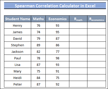
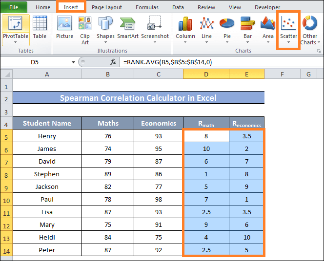
We will use the dataset below for the demonstration. This dataset comprises two sets in data arrays with Math and Economics column headers. We will examine these two column values and calculate the correlation between them.

Spearman rank correlation Calculator Excel

1. Computation of Spearman Correlation Using Excel Formula

Below is an example of a basic Spearman Correlation approximation:

Calculating Spearman Correlation in Excel Using a Traditional Formula, where di is the distinction between two rankings

As for the number of observations, it is n.

If a ranking has tied values, this formulation will not function. We must look at the ranking dataset to see if this approach works well with ours.

The Spearman Correlation Coefficient is computed by first ranking the values applying the RANK.AVG function, and then using those ranks.

Steps

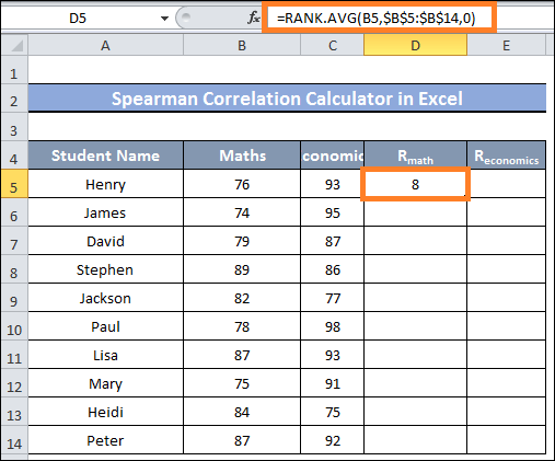
The values in the columns Math & Economics must first be ranked.
In cell D5, type the following formula and hit Enter to accomplish that:

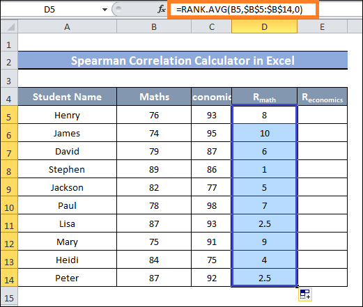
Next, move cell D14 with the Fill Handle.
As you can see, the values in a range of cells D5:D14 have been ranked.
Use the Traditional Equation to compute the Spearman Correlation in Excel.
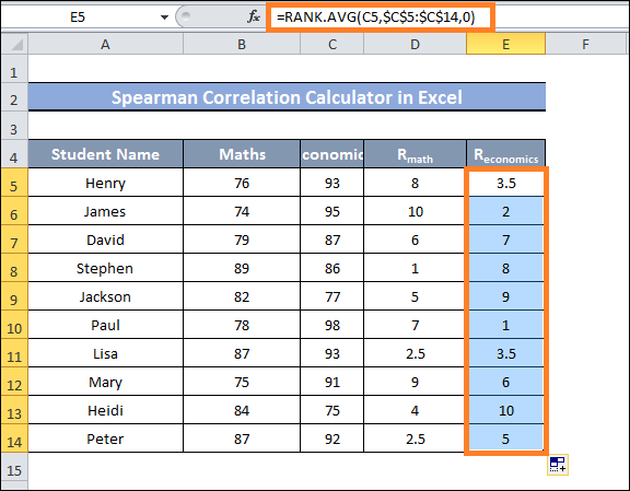
Next, enter and type in the following formula in cell E5 to rank a range of cells C5:C14:

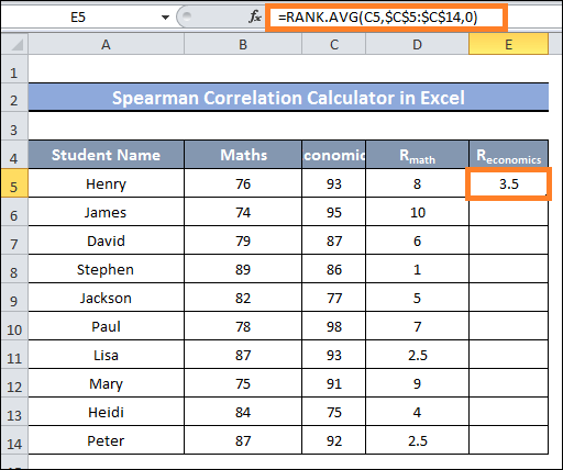
After that, drag cell E14 with the Fill Handle.
You should now see the current ranking of the values in the cells E5-E14 range.
Currently, if we pay close attention, we can see that there are no values with the same rank in the rank of the column values for Math and Economics.
Therefore, calculating the Spearman correlation within the Excel spreadsheet using our method may be done without problems.
Our current task is determining the variation in each row's ranking value.
Simply type the following formula into cell F5 and hit the enter key to accomplish this:

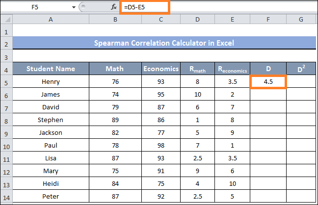
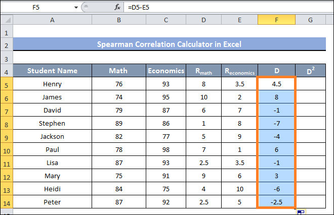
After that, drag cell F14 with the Fill Handle.
You can now see the variations in the ranking values in every row displayed inside the F5-F14 cell range.
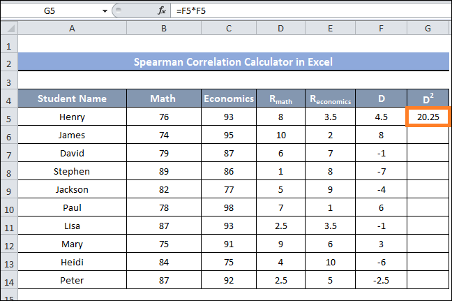
The square for the discrepancy between the ranking values in each row must now be found, and it may be found in cells C5 through C14
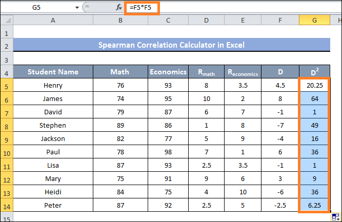
To accomplish this, type the following formula into cell G5 and hit the enter key:

After that, drag cell G14 with the Fill Handle.
You can now see the square of the distinction between each row's rated values for every cell in the range of G5 to G14.
In cell G15, use the following formula to obtain the sum of the ranges of cells G5:G15:

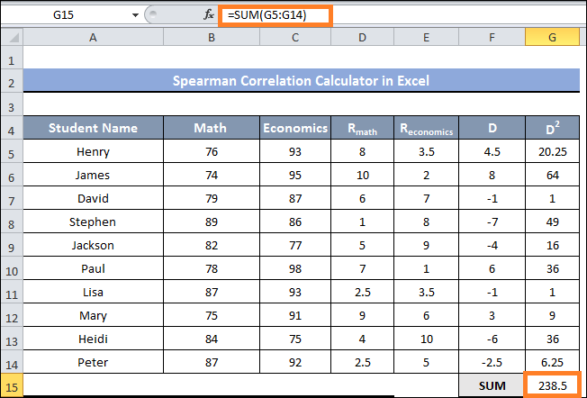
We now have all of the parameters required to calculate the Spearman correlation.
In cell D16, please enter the number for entries; in this instance, it is 10.
Fill in cell D17 with the following formula:

In an instant, you will receive the Spearman Correlation.
There is a negative correlation among the two ranking data columns, as indicated by the output's negative value.
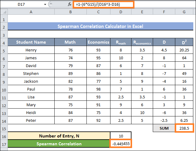
The final result makes it clear that the value we obtained is negative. It suggests a negative relationship between the values within the Math and Economics columns. In other words, if one column's value rises, another will not, and vice versa.

2. Spearman Correlation Calculation Using the CORREL Function

The CORREL function provides the correlation across two cell value ranges. You can use these values to find the correlation among the two ranges of variables. The value falls in the range of -1 to +1. When the value is positive, it means that when one dataset's value rises, another dataset's value rises as well, and vice versa. Additionally, we rank the entries using the RANK.AVG function.

Steps:

Prioritising the values of the Math and Economics columns is necessary initially.
To accomplish it, type the following formula into cell D5 and hit the enter key:

Next, to cell D14, drag the fill handle.
Then, you will see that the values in the range of cells D5:D15 are currently ranked.
Next, enter and hit enter the given formula in cell E5 to rank the distance of cells E5:E14:

After that, drag cell E14 with the Fill Handle.
You will now see a ranking of the data in the cells E5-E14 range.
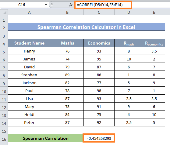
Next, pick cell C17 and type the following equation in it:

Cell C17 now has the Spearman correlation, as you can see after entering the formula.

Calculating the Spearman Correlation How to Use Graph in Excel

The R squared value is simple to compute with a scatter plot, and the Spearman Correlation value may be obtained by simply square rooting the total value. However, adjustments to the value sign may be necessary based on the slope of the Trendline. Before proceeding, the RATE.AVG function is used to rate the data, with the SQRT function applied in this process.

Steps:

The ranking of the Math and Economics columns is necessary.
To achieve this, the values in the Math and Economics columns need to be ordered.
To accomplish it, type the following formula into cell D5 and hit the enter key:

Next, move cell D14 with the Fill Handle.
You will now see that the values within the cells D5 through D14 range are now ranked.
Next, enter and hit enter the given formula in cell E5 to rank the value range of cells E5:E14:

Drag cell E14 with the Fill Handle.
You will observe the data in the range of cells E5 to E14 being ranked.
RMath and REconomics are the two columns we must select to generate a scatter plot using the ranked two columns.
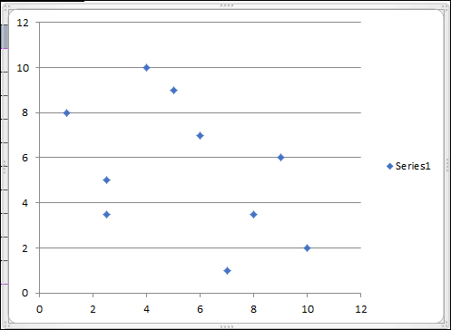
After that, select the Scatter plot by clicking on it from the Insert tab's Charts group.
You will notice that the X- and Y-axes of the chart are accompanied by the values from the RMath column and the REconomics values when a new chart window opens.
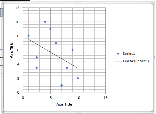
On the chart's side, click the Chart Elements icon now.
To add a trendline to the chart, check the Trendline option.
The chart will display a Trendline pointing downward when you tick the item.
Then, select the histogram-shaped symbol from the trendline option menu.
Next, check the box to display the R-squared value on the chart.
Now, observe the appearance of the R-value on the chart.
Take note of this value.
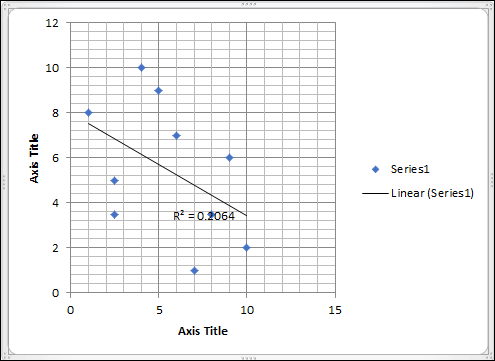
Input the value of R2 in cell D16 after selecting it.
To find the Spearman Correlation value, we must square root that R2 value.
Put the following formula in cell D18:

The final value of the Spearman Correlation in cell D18 requires a small modification. To accomplish this, you must first observe the Trendline's slope. Cell D18's indication should be changed if it is downward. The sign does not need to be changed if a slope is upward.
The Trendline, in this instance, is pointing downward. Therefore, we must change the D18 cell value's sign from 0.41821 to -0.4821.
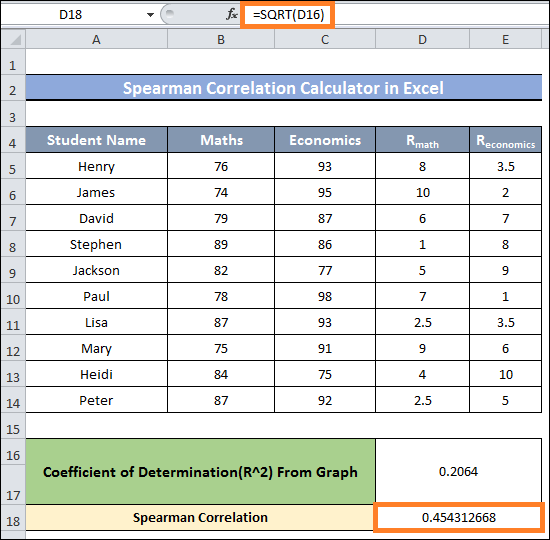
This represents the dataset's final Spearman Correlation value.
A negative value for the final number indicates a negative correlation between the data columns.