How to use the VLOOKUP Function with Choose Function in Microsoft Excel

It was well known that in Microsoft Excel, the respective "VLOOKUP function" is basically a fundamental tool that can be effectively used for the purpose of searching as well as retrieving the selective amount of data from tables that are based upon a specific criterion. It is particularly useful while dealing with the huge sets of data or tables where we need to locate quickly and extract the information effectively. VLOOKUP works by searching for the specific value in the very first column of a specified range (table) and then returning a corresponding value from a designated column within the same row respectively.

Moreover, on the other hand, the respective "CHOOSE function" eventually enhances Microsoft Excel's capabilities by just allowing users to efficiently select a value from a list of options that are based upon a specified position as well as the index. Despite this function, it is quite essential to create a dynamic list of choices, thus enabling particular users to pick up the desired value that is based upon certain conditions as well as specific criteria.

However, by combining the two important functions on Excel- the "VLOOKUP" function and the "CHOOSE" function- the respective users can easily create more flexible and adaptable formulas.

• For example, As an example let us assume that we have a table that usually contains the relevant information regarding the employees who are actually working in the company named "BBPPL," where the department of each employee is primarily stored in the different columns which are effectively based upon their location as well. Instead of manually adjusting the respective column index in the VLOOKUP formula each time, we can make use of the CHOOSE function in order to dynamically select the appropriate column index that is based on the location of the particular employee effectively.

This dynamic approach will not only streamline the process but will also reduce the chances of getting errors and hence make the respective spreadsheet more robust to make effective changes in it. And spite of all this, it will also allow Excel users to build more sophisticated lookup formulas that can automatically adjust to the different scenarios without requiring any constant manual intervention effectively, and the effective combination of the "VLOOKUP" and "CHOOSE" functions in Microsoft Excel empowers users to easily create efficient and adaptable lookup formulas, that are responsible for the purpose of enhancing out the functionality and the versatility of their spreadsheets while dealing with the complex datasets and varying conditions as well.

What is meant by the term "Vlookup" function in Microsoft Excel?

In Microsoft Excel, the "VLOOKUP" Excel function is primarily used for the purpose of searching out the particular value and is also responsible for the purpose of returning a corresponding match, which is based upon a unique identifier respectively. A unique identifier is uniquely associated with all the records of the database. For instance, employee ID, student roll number, customer contact number, seller email address, etc., are unique identifiers as well.

• For example, Let us now suppose that we have a dataset of the employee salaries that are none other than $250, $400, $700, and $1000 from cell B2:B5 and employee ID (1001,1002,1003,1004) that range from the cell A2 to A5. Then, in the cell E2, and despite this, we actually want to know the ID of the respective for the salary of $400, which is in cell B3. In such a scenario, we can now efficiently make use of the VLOOKUP function. And then, inserting out the lookup_value in the cell D2, and here we can now enter the formula as follows:

And just after applying the above formula, it will return the output as "1002." In simple words, a particular user may use the "VLOOKUP" formula in order to search specific information (such as employee ID) in an Excel database (table in Excel worksheet) and find information which is associated with the salary of the employee's salary with it. And more often, the "V" in VLOOKUP usually stands for the vertical. This function mainly looks for a search value in the very first column (lookup column) of the specified range and is also responsible for the purpose of returning a match from the same row of the other column (return column).

What is the syntax for the Vlookup Function in Microsoft Excel?

The syntax of the VLOOKUP Function that can be efficiently used by an individual in an Excel sheet is as follows:

Here, in this particular syntax, the function usually accepts four basic arguments that are none other than the following ones:

Moreover, in the above syntax the very first three arguments are considered as the mandatory one, while the last one is termed to be an optional one as well. Now let us get a brief about the arguments.

1. lookup_value: The lookup_value in the Vlookup function is primarily considered mandatory argument, as it mainly represents the value we actually want to look up in the first column of the selected table or the dataset.
2. table_array: The table array in the Vlookup function is also considered as a mandatory argument. It basically represents the dataset or data array that needs to be searched out effectively.
3. col_index_num: The col_index_num in the Vlookup function is considered as the mandatory argument as it represents the integer which is responsible for the purpose of specifying the column number of the respective table_array that we actually want to return a value from respectively.
4. range_lookup: The range_lookup in the Vlookup function is considered as the optional argument, and it represents or can define what the function should return if it does not find an exact match to the lookup_value as well. Despite all this, this particular argument can be set to "FALSE" or "TRUE," in which the TRUE value usually indicates an approximate match (it makes use of the closest match below the lookup_value in case the exact match is not found), and "FALSE" value indicates an exact match (and it primarily returns an error in case the exact match is not found). "TRUE" can also be substituted for the value of "1," and "FALSE" can be altered for "0,"

How can one easily make use of the Vlookup Function in Microsoft Excel?

Now, in this section, we will go through some of the examples of the VLOOKUP function used in Microsoft Excel. They could be quite beneficial for both beginners and also for advanced Excel users respectively:

#Example 1:

Now, for this example, we will be constructing a table with the data that depicts the prices for the various types of dresses worn by newborn babies. And for this, we actually want to find out the price of the dresses like Romper, Mini-skirt, Pant, T-shirt, Frock as well.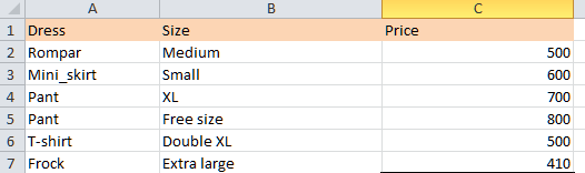

The steps that are required to make use of the VLOOKUP Excel function in an Excel sheet are listed below, and we need to follow them sequentially:

Step 1: First of all, we are required to organize the selected data in the left to the right format it due to the reason that, the respective Vlookup function works in this order as well. Such an arrangement has been efficiently depicted in the following image, making it easy to make use of the VLOOKUP function.

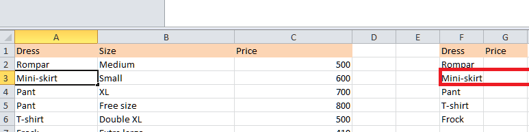
Step 2: In this step, we are required to place the cursor where the formula needs to be entered.

• For example, in this example, we need to find out the price of the Mini-skirt, and in this, we need to place the cursor in cell G3, as it was clearly depicted in the next image.

Step 2: In this step, we must enter the formula "=VLOOKUP(F3,B1:C7,3,FALSE). " This formula is essential for supplying the correct arguments to the function and finding the exact value.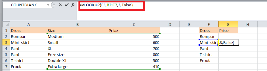

In the following pointers, starting from steps 3a to 3d, all the respective arguments of the "VLOOKUP" function regarding the current example are explained effectively one by one.

Step 3(a): Lookup_value: Lookup_value is the function's first and main argument. It primarily specifies the value that needs to be searched in the table. So, the particular "lookup_value" is F3 (mini-skirt).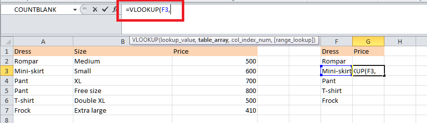

Step 3(b): Table_array: And now the table_array in this formula usually refers to the table range in which the respective lookup value needs to be searched out. So, the lookup value is to be searched in the ranges that range from cell B1 to cell C7 of the lookup table.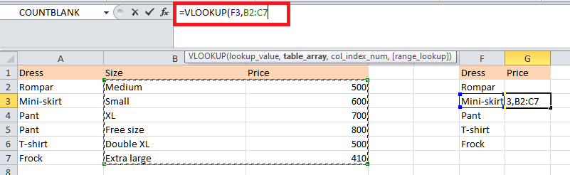

Step 3(c): Col_index_num: Col_index_num is the index number of the column, and it mainly specifies the column from which the respective value needs to be returned.

• For example, here in this part, the word "mini-skirt" is primarily present in the column.
• B(Column 3). Now, this argument is 3 and refers to the second column of the table array.

Note: It should be noted that the leftmost column of the table array is effectively counted as 1.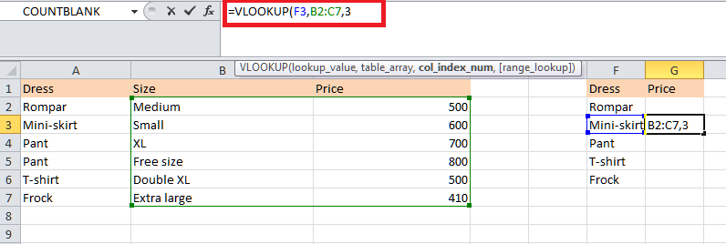

Step 3(d): Range_lookup: The Range_lookup is termed to be the Boolean value that yields "True" or "False." The values are explained as follows respectively:

• True - It is mainly used for an approximate or also for the exact close match. And the data is also matched with the argument approximately. For instance, the first word is mainly looked up if the selected data contains more than one word as well.
• False - It is primarily used for an exact match. All the words in the data are matched, and the corresponding value is returned effectively.

Hence, after that, we are required to enter the "False" value because we actually want the formula to return an exact match. The complete formula is depicted below in the next image.

Note: The default value is " True " if the "range_lookup" argument is omitted.

Step 4: In this step, we are required to press the "Enter" key from our respective keyboards. All the arguments are usually passed correctly. The result is mainly displayed in the following image as well.

Step 5: After performing the above steps, we are required to drag out the formula in order to obtain the prices of the T-shirt, Romper, Frock as well as the dress. The output is mainly depicted in the following image.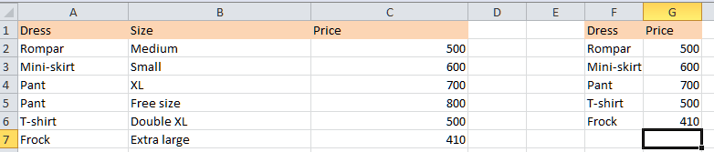

#Example 2

Now, in this example, the respective following table usually depicts the marks of the 6 students in the various subjects as well. The serial ID (Sid) number is in the first column (A) respectively.

So, in this, we are required to find out the marks that correspond to the serial ID numbers 4 and 8.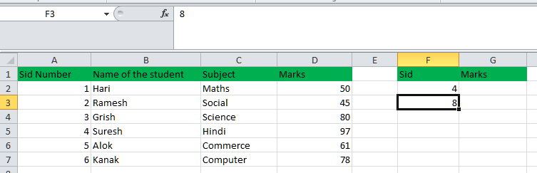

More often, the respective steps that can be easily applied to the VLOOKUP function are mentioned below effectively:

Step 1: First, we must organize the data and place the cursor in cell G2, where we actually want to enter the formula.

Step 2: After that, we must enter the VLOOKUP Excel formula in the selected cell G2. To auto-populate the formula, we need to press the "tab" key.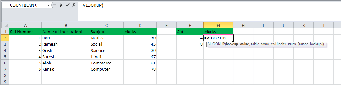

Step 3: In this step, we must enter the function's first argument, as it is depicted clearly in the next image. The "lookup_value" is cell F2. It is the value we are looking for.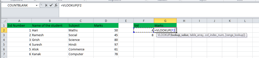

Step 4: After that, we need to enter the next argument, the table_array. Then, we need to select the cells ranging from cell A1 to cell D7, as shown in the following image. It is the source table where the serial ID is to be found effectively.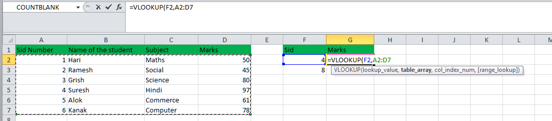

Step 5: Then, we must enter the col_index_num, the serial number of the column from which the value needs to be returned. Since we want the function to return a value from the "marks" column, we are required to type 4. The serial ID number column (A) is counted as 1, respectively.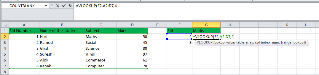

Step 6: Now, in this step, we just need to enter the argument "range_lookup," which consists of the two values that are none other than "True" or "False." Since the latter value returns an exact match, we need to type "False." Finally, close the brackets of the formula. And the exact match option (False) is usually used to the avoid confusion. The complete formula is as shown in the following image.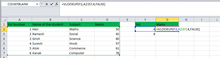

Step 7: Now, in this step, we need to press the "Enter" key from our respective keyboard as the formula is ready to be applied, and the output is efficiently depicted in the following image. Just after that, we need to drag the formula of cell G2 in order to obtain the result in cell G3 respectively.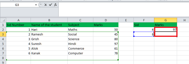

What is meant by Choose Function in Microsoft Excel?

It was well known that the respective "CHOOSE" Function in Microsoft Excel returns a value from the given range of the data that is also considered as the "array" when the position that is "index" is mainly specified by the particular user. This lookup, as well as the reference function of Microsoft Excel, is most commonly used for the purpose of creating scenarios in financial models.

More often, the respective CHOOSE function in Microsoft Excel is like having a menu card where we actually want to pick out exactly what we want. Let us imagine that we have a list of the options, such as different dishes on a menu card available at a particular restaurant. With the CHOOSE function, we are telling Excel to select the specific option from that particular list based on a number we have provided.

• For example: Let's assume that we have a list of potential investments with their respective returns, such as stocks, bonds, as well as real estate. By making use of the CHOOSE function, we can easily tell Microsoft Excel to pick the investment options that are based on a number that we give it. If in case we enter the number 3, then it will choose real estate; for 1, it will select stocks and vice versa.

However, this function is particularly handy in financial models where we might want to explore the various scenarios as well, and thus, by making use of the CHOOSE function, we can easily switch between various options or the scenarios within our model and thus making it more dynamic as well as the adaptable to the different situations. If in case we are analyzing different investment strategies or forecasting financial outcomes, the CHOOSE function in Microsoft Excel will help us to quickly assess the impact of each scenario without manually changing a bunch of the cells effectively.

What is the syntax of the CHOOSE function in Microsoft Excel?

The syntax of the CHOOSE Function that can be efficiently used by an individual in an Excel sheet is as follows: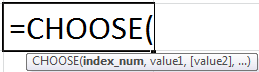

The respective CHOOSE function in Microsoft Excel primarily accepts the following arguments which are as follows:

1 - Index_num: The Index_num argument is the position of the value to choose from, and despite this, it is mainly a number that lies between 1 and 254. It can also be a cell reference or a function which are responsible for giving a numerical value. It can be in any of the following forms as well:

• 5
• B2
• "=RANDBETWEEN(4,10)"

Note: It should be noted that if "Index_num" is manually entered as a fraction, then in that particular scenario, it will be efficiently truncated to the lowest integer at the time of use effectively.

2: Value1, [value2], [value3]: This could be the list of the data from which a particular value needs to be returned. More often, it could be a set of numbers, cell references, cell references in the form of arrays, text, formulas, as well as functions. It could be in any of the following forms which are as follows:

• 1, 2, 3, 4, 5
• Monday, Tuesday, Wednesday
• A8, A10, A12
• A3:A5, B7:B9, C11:C13, D5:D7

The "Index_num" and the "value1" are mandatory arguments. The rest of the arguments are optional.

How can one easily make use of the CHOOSE function in Microsoft Excel?

Let us now consider the following examples for a better understanding of the CHOOSE function in Microsoft Excel:

# Example 1

For this example, we have considered 8 data points, which are as -2, 3, 10, 24, 8, and 11, 5, 12, and from this, we actually want to choose the 5^th element as well. Now, for this, we need to apply the formula as "=CHOOSE(4,2,3,10,24,8,11,5,12)" or "=CHOOSE(4, A3, A4, A5, A6, A7, A8)."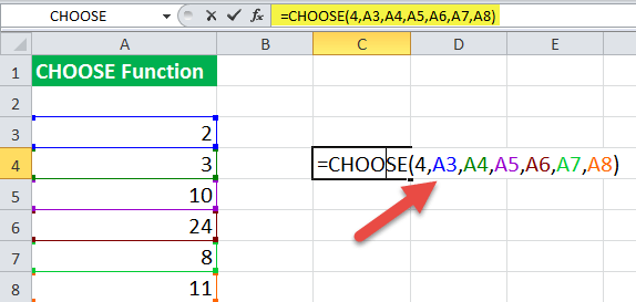

By just applying the above formula, it will return the output as cell 24. If cell A4 is selected as the index value, then in that case it will return the output as 10. It is because of the reason that, the respective A4 corresponds to 3. The third value in the dataset is A5, i.e., 10 respectively.

#Example 2:

For this example, we generally have three columns, each containing a list of fruits and flowers and their numbers. We want to choose a value from the array of values. Let us suppose that we want to choose the third value.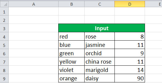

Now, after that, we need to apply the CHOOSE formula in an Excel sheet respectively.

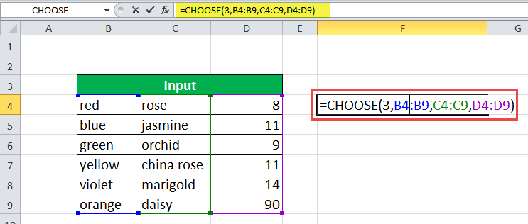
It could be seen that the third value is a list of the values that range in the cell "D4:D9," and which is quite greater than or equal to the input values of column D (8, 11, 9,11,14,90). So, the output of the formula will remain the same as the list of the values available in the cell ranging from cell D4 to cell D9, respectively.

Despite all this, in a single cell, the particular formula used will return only a single value as an output from the given list. This selection is not random, as it depends upon the position of the cell in which the answer is required.

And similarly, in cell F4, the respective formula "=CHOOSE (3, B4:B9, C4:C9, D4:D9)" gives the output as 8, which corresponds to the value available in the cell D4, in the same manner in the cell F5, the same input gives output as 11, that mainly corresponds to the value that is available in the cell D5 as well.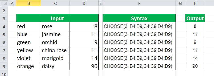

# Example 3:

Now, we will add one more column to our respective input of the previous example. After that, we are required to apply the following formula to effectively choose the fourth value from the given list of values.

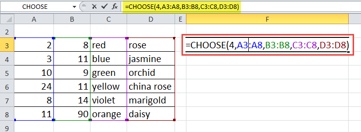
After proceeding with the above formula, we will encounter the output shown in the succeeding image as well.

How can one easily make use of the Vlookup function in combination with the Choose function in Microsoft Excel?

In the above section, we learned about both functions in detail with the help of different examples. Now, we will understand the combination of VLOOKUP with the CHOOSE functions with the help of the following examples.

# Example 1: Combining out the Microsoft Excel VLOOKUP functions and CHOOSE function for the Single Condition.

Now, in this particular example, we will be effectively working with the 1 condition in order to make use of the VLOOKUP in combination with the CHOOSE functions. For this part, we have prepared the dataset as well, and this dataset will depict the set of Marks Obtained that have a strong relation to the Grade Obtained and also with the Remarks of an exam.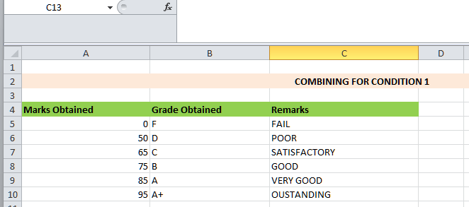

Now, after that, we will be combining both functions for a single condition.

1. First of all, we need to type the number 78 in cell B14 as the condition.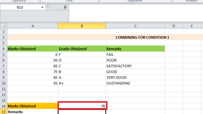

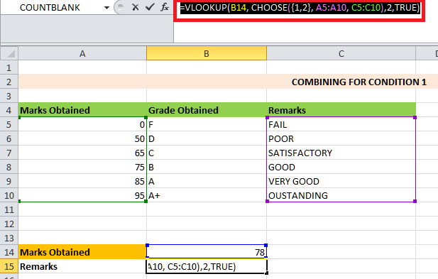
2. Then, we will insert the formula below in cell B15.

3. And just after entering the above formula into cell B15, we are required to hit the Enter key on our keyboard.

4. That's it, and then we will able to get the look-up value for the 1 Condition effectively.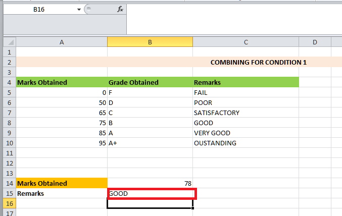

More often, in this particular formula, the respective VLOOKUP function is mainly used for the purpose of looking up the value in cell B13. Then, CHOOSE ({1,2}, A5:A10, C5:C10) is used as the table range where {1,2} means it will display 1 or 2 as the index_num argument. Following type 2 as the col_num argument for the VLOOKUP function. And at last, we will be inserting the TRUE for an approximate match respectively.

Now, to have the proof check, we will change the condition value in cell B12, and the output will be changed automatically as the condition value changes.

# Example 2: Applying the VLOOKUP function with the CHOOSE function for 2 Conditions in an Excel sheet.

We all knew that, the respective combination of the VLOOKUP as well as the CHOOSE functions can also work in a similar pattern for the 2 Conditions. So, in order to get better insight, we need to follow the below-mentioned steps respectively:

1. First, we are required to prepare a dataset with the following information, which is mentioned below in the table.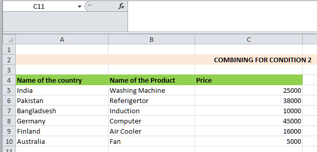

2. Now, just after the collection of the data, we are required to type Germany and Computer as the conditions in the cells none other than cell B12 and B13, respectively.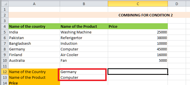

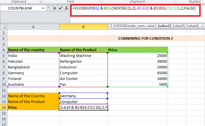
3. Afterward, we need to type this formula in cell B14.

4. And last, we are required to press the Enter key from our respective keyboard

5. Finally, we will see the value that actually meets our specified conditions.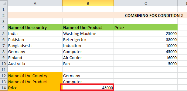

However, here in this particular example the VLOOKUP function is mainly used for the purpose of looking for the value in the cells that are none other than the cells B12 and B13. And after that, the respective CHOOSE({1,2}, A5:A10&B5:B10, C5:C10) can be effectively used as the table_range where {1,2} means it will be displaying 1 or 2 as index_num argument. Following type 2 as the col_num argument for the VLOOKUP function. Lastly, we can insert TRUE for an approximate match as well.

# Example 3: Insertion of the VLOOKUP function with the CHOOSE function for 3 Conditions

Now, just like the 2 conditions, in this example, we can simply insert the VLOOKUP function in combination with the CHOOSE function for 3 conditions. To achieve this, we must go through the steps below effectively.

1. We are required to prepare a dataset ranging from cell A4:D10with the following information.

2.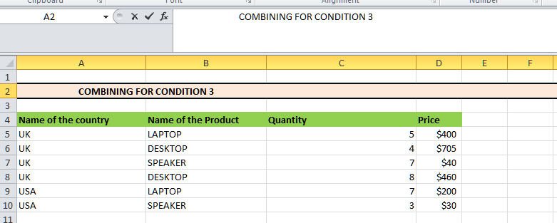

3. In this step, we are required to typeUSA, Laptop, and 7 as the 3 conditions.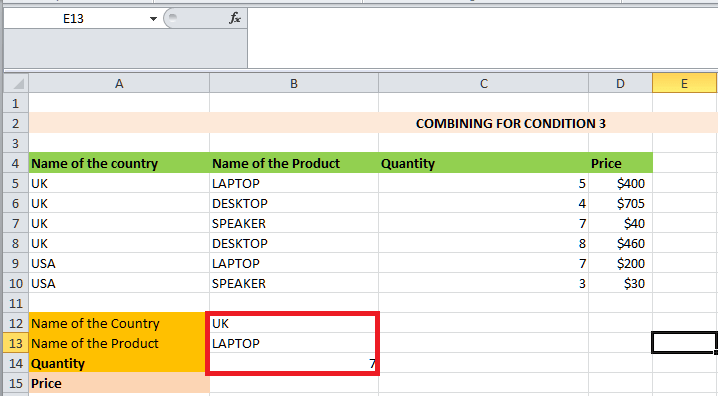

4. Now, after that, we need to apply this formula in cellB15.

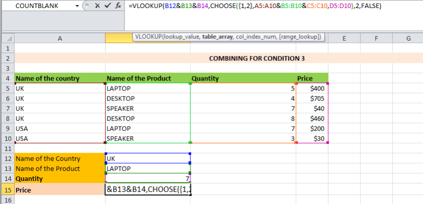
5. Finally, we are required to hit the Enter key from our respective Keyboard, and we will see the required value depicted in the table below as well.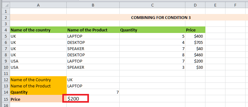

More often, in the formula mentioned above, the respective VLOOKUP function is mainly used to look for the value in the cells that are none other than cells B12, B13, and B14. And after that, we are required to use CHOOSE({1,2}, A5:A10&B5:B10, C5:C10,D5:D10) as the table_range where {1,2} means that it stands for 1 and 2 as the index arguments.

What are the key takeaways regarding the use of the Vlookup function with the choose function in Microsoft Excel?

The important key points which need to be remembered by an individual while working with the Vlookup function in combination with Choose function in Microsoft Excel are as follows:

1. Main purpose: The respective `VLOOKUP` function in Microsoft Excel is primarily used for the purpose of finding out a value in the very first column containing table of array, and it would be returning a value in the same row from the selected column, And on the same way the `CHOOSE` function is employed for the purpose of returning out a value from a list of the values which are eventually based upon a specified index number respectively.

2. Doing the setup of the data: Here in this, we are required to ensure that our respective data is basically organized in the proper sequence as well. More often, for the `VLOOKUP,` the respective lookup value must need to be in the first column of the table array. And for the `CHOOSE`, we must need to have a list of the values that are ready to be selected from in an effective manner.

4. Index numbers: We must ensure that the index numbers used in the `CHOOSE` function match the column index number we actually want to retrieve with the `VLOOKUP` function.