| |

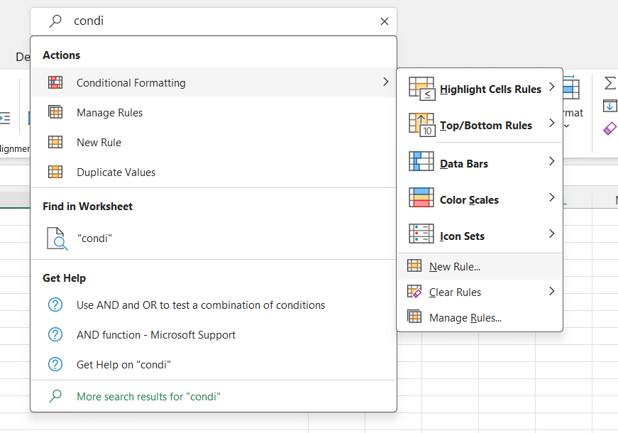
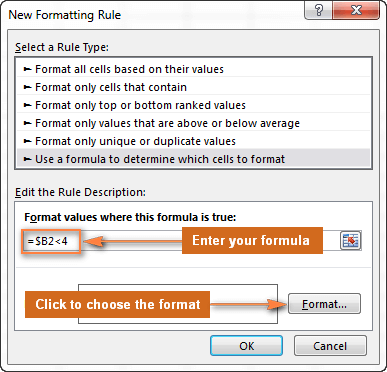
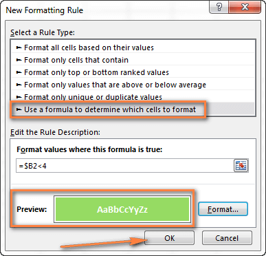
GOOGLE SHEETS CONDITIONAL FORMATTING ON ANOTHER CELLIntroduction:Excel restrictive organizing in view of another cell esteem Excel's predefined restrictive organizing, for example, Information Bars, Variety Scales and Symbol Sets, are chiefly purposed to arrange cells in light of their own qualities. To apply restrictive designing in view of one more cell or configuration a whole line in light of a solitary cell's worth, then you should utilize recipes. In this way, we should perceive how you can make a standard utilizing an equation and after examine recipe models for explicit undertakings. How to create a conditional formatting rule based on formula:To set up a restrictive designing principle in light of an equation in any variant of Succeed 2010 through Succeed 365, do these means:
NOTE: Whenever you really want to alter a contingent designing equation, press F2 and afterward move to the required spot inside the recipe utilizing the bolt keys. In the event that you have a go at arrowing without squeezing F2, a reach will be embedded into the recipe as opposed to simply moving the addition pointer. To add a specific cell reference to the equation, press F2 a subsequent time and afterward click that cell.Excel contingent designing recipe models: Since it is now so obvious how to make and apply Excel contingent organizing in light of another cell, how about we continue on and perceive how to utilize different Succeed recipes by and by.
Equations to look at values (numbers and text) As you most likely are aware Microsoft Excel gives a small bunch of prepared to-utilize rules to design cells with values more prominent than, not exactly or equivalent to the worth you determine (Restrictive Organizing >Highlight Cells Rules). Be that as it may, these standards don't work if you need to restrictively design specific segments or whole lines in light of a cell's worth in another section. For this situation, you utilize comparable to recipes:
The screen capture beneath shows an illustration of the More prominent than recipe that features item names in segment An if the quantity of things in stock (section C) is more prominent than 0. If it's not too much trouble, focus that the equation applies to section A main ($A$2:$A$8). However, assuming you select the entire table (for our situation, $A$2:$E$8), this will feature whole lines in view of the worth in section C. 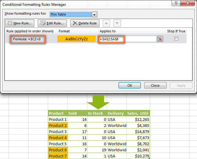
Likewise, you can make a contingent designing standard to look at upsides of two cells. For instance:
As you can find in the screen capture underneath, these recipes work for text values as well with respect to numbers. 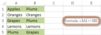
What's more, as well as recipes If you have any desire to arrange your Succeed table in light of at least 2 circumstances, then use either =AND or =OR capability:
In the screen capture underneath, we utilize the recipe =AND($C2>0, $D2="Worldwide") to change the foundation shade of lines if the quantity of things in stock (Segment C) is more prominent than 0 and assuming the item sends around the world (Section D). If it's not too much trouble, focus that the equation works with text values as well similarly as with numbers. Normally, you can utilize two, three or more circumstances in your AND as well as equations. To perceive how this functions practically speaking, watch Video: Restrictive organizing in view of another phone. These are the essential restrictive arranging equations you use in Succeed. Presently we should think about somewhat more complicated yet undeniably additional fascinating models. Restrictive organizing for void and non-void cells I think everybody knows how to design vacant and not unfilled cells in Succeed - you just make another standard of the "Arrangement just cells that contain" type and pick Spaces or No Spaces. A standard to organize clear and non-clear cells in Excel 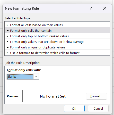
However, imagine a scenario where you need to design cells in a specific section in the event that a relating cell in another segment is unfilled or not vacant. For this situation, you should use Excel equations once more: Equation for spaces: =$B2="" - design chosen cells/lines in the event that a comparing cell in Segment B is clear. Recipe for non-spaces: =$B2<>"" - design chosen cells/lines in the event that a comparing cell in Segment B isn't clear. NOTE: The recipes above will work for cells that are "outwardly" unfilled or not vacant. Assuming you utilize some Succeed capability that profits a vacant string, for example =if(false,"OK", ""), and you don't maintain that such cells should be treated as spaces, utilize the accompanying equations rather =isblank(A1)=true or =isblank(A1)=false to design clear and non-clear cells, separately.Example: Also, here is an illustration of how you can involve the above equations practically speaking. Assume, you have a section (B) which is "Date of Offer" and another segment (C) "Conveyance". These 2 sections have a worth provided that a deal has been made and the thing conveyed. Thus, you believe that the whole column should become orange when you've made a deal; and when a thing is conveyed, a relating line ought to become green. To accomplish this, you really want to make 2 contingent arranging rules with the accompanying equations:
Another thing for you to do is to move the second rule to the top and select the Stop assuming genuine really take a look at box close to this standard: 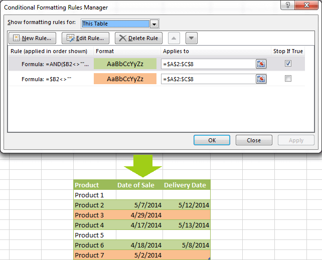
In this specific case, the "Stop if valid" choice is really pointless, and the standard will work regardless of it. You might need to check this crate similarly as an additional safeguard, on the off chance that you add a couple of different guidelines later on that might struggle with any of the current ones.
Next TopicHow to Color Alternate Rows in Excel
|
 For Videos Join Our Youtube Channel: Join Now
Feedback
- Send your Feedback to [email protected]
Help Others, Please Share


