| |

Loan Amortization Schedule in ExcelAn amortising loan is simply a fancy phrase for a loan with instalment payments due for the duration of the loan. In essence, every loan amortises in some manner. For instance, there would be 12 regular instalments for a loan with full amortisation over 12 months. Part of each payment goes towards interest, and part goes towards the Principal. You can create a loan amortisation schedule that details all loan payments. An amortisation schedule is a table that displays the remaining balance following each payment, breaks down each instalment in interest and Principal, and details the periodic payments of a loan/mortgage over time. How to make an Excel loan amortisation scheduleUsing the following Excel functions, we can create a mortgage or loan amortisation schedule:
Let's now walk through each phase of the procedure. 1. Establish the amortisation scheduleTo begin with, specify the input cells that will include the known loan components:
The next step is making an amortisation table with the labels Period, Payment, Interest, Principal, and Balance in B9:F9. Enter a string of numbers in the Period column (1-12 in this example) that represent the total number of payments: 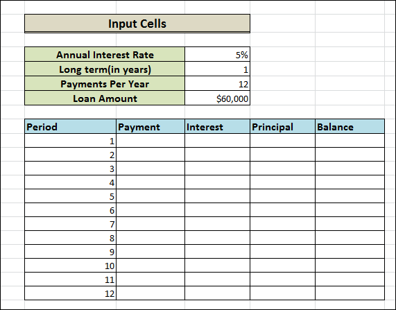
Now that we have established all the necessary elements, let's move on to the most fascinating aspect: loan amortisation calculations. 2. Use the PMT formula to determine the total payment amount.A PMT(rate, nper, pv, [fv], [type]) method is used to determine the payment amount. It would help if you used consistent values for the rate and nper parameters to handle various payment frequencies (weekly, monthly, quarterly, etc.) correctly:
Combining the arguments above yields the following formula: = PMT($D$4/$D$6,$D$5*$D$6,$D$7)
We use absolute cell references since this formula should automatically copy to the cells below. When you input the PMT formula into C10 and drag it along the column, the payment amount for each period will remain the same: 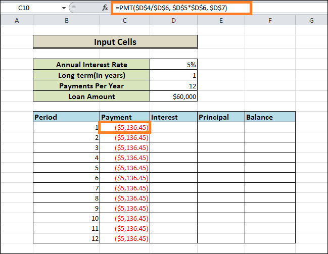
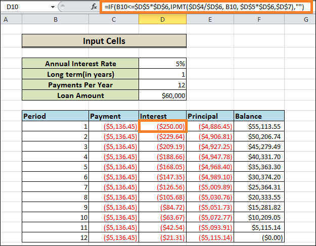
3. Use the IPMT formula to calculate interestEach periodic payment's interest component can be found using an IPMT(rate, per, nper, pv, [fv], [type]) function: =IPMT($D$4/$D$6, B10, $D$5*$D$6,$D$7)
All arguments within the PMT formula are identical, except the payment period-specific per argument. This input is provided via a relative cell reference (B10) because it is expected to vary according to the relative position of the row that the formula is copied to. After copying this formula down to D10, you can use it in the same number of cells as necessary: 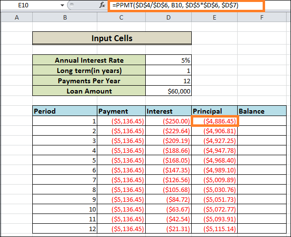
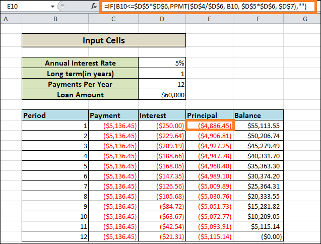
4. Use the PPMT formula to find the PrincipalUse the following PPMT formula to determine the principal portion of each periodic payment: = PPMT($D$4/$D$6, B10 ,$D$5*$D$6, $D$7)
The arguments and syntax are precisely identical as in the previously mentioned IPMT formula: This formula starts in E10 and goes up to column E. To calculate the principal amount of a loan's periodic payments, use the PPMT formula. 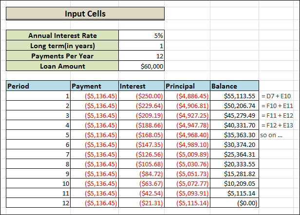
Here's a tip: sum the amounts in the Principal & Interest columns to see if your calculations are correct. The total should match the amount in the Payment column in the same row. 5. Obtain the remaining BalanceTwo separate formulas will determine the remaining balance for each period. Add the loan amount (D7) with the first period's principle (E10) to determine the balance in F10 following the first payment: = D7+E10
The Principal is really deducted from the loan amount as it is a negative number, while the loan amount is a positive number. Add the Principal for this period to the preceding balance for the following and all subsequent periods: = F10+E11
The formula above is copied along the column and goes up to F11. The formula makes the appropriate adjustments for every row because relative cell references are used. And that's it! We have completed our monthly loan amortisation programme. 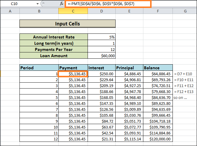
Tip: Provide payments that are positive figures Excel functions display the payment, interest, and Principal as negative amounts since loans are paid from your bank account. The graphic illustrates how certain values are, by default, highlighted with red and surrounded by parenthesis. A negative sign should be used before the PMT, IPMT, and PPMT functions if you would rather have all returns as positive numbers. Instead of adding, use subtraction for the Balance formulae, as the screenshot below illustrates: 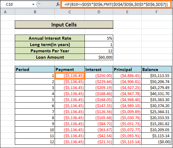
Amortisation Schedule for a variable number of periodsIn the example above, we created a loan amortisation schedule for the predetermined number of payment terms. For a particular loan or mortgage, this simple one-time fix is effective. A more thorough technique is required to design a reusable amortisation schedule using a variable number for periods, as explained below. 1. Enter the maximum number of periodsPut the maximum payments you will accept for any loan within the Period column. To input a number sequence more quickly, use Excel's AutoFill tool. 2. In amortisation calculations, use IF statements.It would help if you found a way to restrict the computations to the true amount of payments due for a certain loan, as you now have a lot of inflated period numbers. To achieve this, enclose each formula in an IF statement. The IF statement's logical test determines if a period number within that row equals or is less than the total payments. The empty string gets returned if the result of the logical test is FALSE; if it is TRUE, the associated function is calculated. The following formulas should be entered in the respective cells, assuming that Period 1 is in row 8. These should then be copied throughout the entire table. Payment (C10): =IF(B10<=$D$5*$D$6,PMT($D$4/$D$6, $D$5*$D$6, $D$7))
Interest (D10): =IF(B10<=$D$5*$D$6,IPMT($D$4/$D$6,B10,$D$5*$D$6,$D$7), "")
Principal (E10): =IF(B10<=$D$5*$D$6,PPMT($D$4/$D$6, B10, $D$5*$D$6, $D$7), "")
Balance: The formula of Period 1 (F10) is the same as it was in the earlier example: = D7+E10
The formula looks like this in Period 2 (F12) as well as later periods: =IF(B10<=$D$5*$D$6, F10+E10, "")
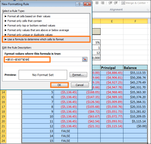
Consequently, you will obtain an accurately computed amortisation plan and numerous blank rows containing the period numbers following loan payback. 3. Hide unnecessary period numbersConsider the work completed and move on to the next stage if you can tolerate seeing unnecessary period numbers shown following the most recent payment. Creating a conditional formatting rule that alters the font colour to white for any rows following the last payment is completed will help you conceal any unneeded periods if you aim for perfection. To accomplish this, choose the Home tab > Conditional formatting > New Rule... > after selecting all the data rows in your amortisation table. Work out which cells to arrange using a formula. To verify whether the period number within column B exceeds the total number of payments, put the following formula in the relevant box: =$B$10>$D$5*$D$6
An important reminder: Make sure you multiply the cells corresponding to the Loan term and Payments per year ($D$5*$D$6) using absolute cell references for the conditional formatting formula to function properly. You apply a combination of a cell reference ($B$10), which is an absolute column and a relative row, to compare the product against the Period 1 cell. 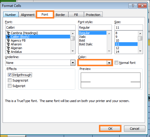
Next, select the white font colour by clicking the Format... option. Completed! Change the font colour to white for any rows that come beyond the final payment period. 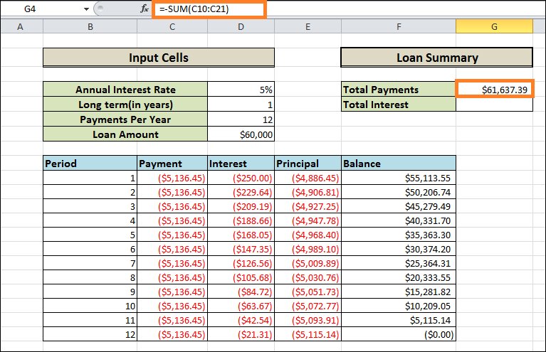
4. Create a Summary of the loanAdd a few extra formulas at the top of your amortisation schedule so that you can quickly examine the summary information regarding your loan. Total Payments(G4): =-SUM(C10:C21)
Total Interest(G5): =-SUM(D10:D21)
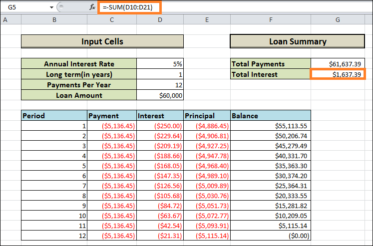
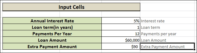
In the formulas above, delete the minus sign if your payments are positive numbers. And that's it! We are ready to proceed with our finished loan amortisation programme! How to use Excel to create a loan amortisation Schedule with Extra PaymentsHopefully, the amortisation schedules covered in the earlier examples are simple to make and follow. They do not, however, provide a helpful feature that many borrowers would find appealing: the ability to make extra payments to expedite loan repayment. This example will examine making a loan amortization schedule with extra payments. 1. Declare the input cellsStart by configuring the input cells as usual. For the purpose of making our formulas simpler to read, let's call these cells as follows:
2. Determine a payment scheduleThe scheduled payment amount, or the amount owed on a loan if no additional payments are made, is a preset cell needed in addition to the input cells for our additional computations. We use the following formula to determine this amount: =IFERROR(-PMT(Interest Rate/Payments Per Year, Loan Term*Payments Per Year, Loan Amount), "")
(Or) =IFERROR(-PMT(D4/D6,D5*D6,D7), "")
Please note that to have a positive result, we have to place a minus sign before the PMT function. We encapsulate the PMT formula inside the IFERROR function to prevent problems if some input cells are empty. Put this formula in a cell (let's use H4) and give it Schedule Payment. Determine the amount to be paid on time. 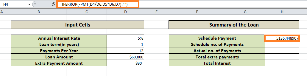
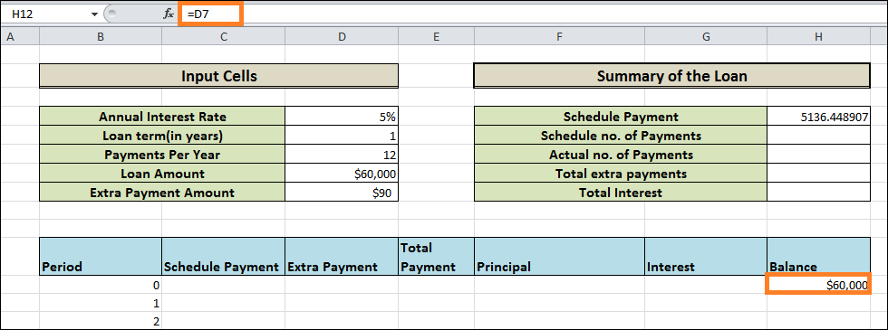
3. Establish the amortization tableWith the headings from the screenshot below, create a loan amortisation table. Put a string of integers in the Period column that starts using zero (since you may conceal the Period 0 row later when necessary). Enter the maximum number of payment periods that can be entered if you want to build a reusable amortization schedule. Select the balance value corresponding to the initial loan amount in Period 0. This row's remaining cells will all remain empty: The formula for H12: =D7
4. Create calculations for an amortisation schedule that includes Extra payments.This is a crucial aspect of what we do. We must perform all the maths since Excel's built-in functions cannot be used for further payments. Note: In this illustration, row 12 corresponds to Period 0 and row 13 to Period 1. Please be careful to change the cell references if the beginning of your amortisation table is in a different row.After entering the following formulas on row 13 (Period 1), repeat the process for each subsequent period. Schedule Payment (C13): Use the scheduled payment if the amount (designated as cell H4) of the scheduled payment is less than or equal to the remaining balance (H12). If not, include the interest from the prior month and the leftover amount. =IFERROR(IF(Schedule Payment<=H12, Schedule Payment, H12+H12*Interest Rate/Payments Per Year), "")
We use the IFERROR function to encapsulate this formula and all others as an additional safety measure. If certain input cells are empty / contain invalid data, this will stop many errors. Extra Payment (D13): Apply the following logic to an IF formula: You should refund the ExtraPayment if it is less than the distinction between the Principal for this period (H12-F13) and the remaining balance. If not, you should use the difference. =IFERROR(IF(Extra Payment<H12-F13, Extra Payment, H12-F13), "")
As a helpful hint, enter any variable amount you have for additional payments directly within the Extra Payment section. Total Payment (E13) Add the extra payment (D13) at the current period and the scheduled payment (C13), and that's all: =IFERROR(C13+D13, "")
Principal (F13) The lesser of the two values-scheduled payment minus interests (C13-G13) or as the remaining balance (H12)-should be returned if the scheduled payment for a given period is larger than zero; return zero otherwise. =IFERROR(IF(C13>0, MIN(C13-G13, H12), 0), "")
It should be noted that the Principal only represents the portion of the regular payment-not the additional payment-that is applied to the Principal of the loan. Interest (G13) Divide the yearly interest rate (cell D4) by the total number of payments made (cell D4), and multiply the result by the amount due at the end of the previous period when the scheduled payment of that period is not zero. If it is, return 0. =IFERROR(IF(C13>0, Interest Rate/Payments Per Year*H12, 0), "")
Balance (H13) Subtract the principal amount for the payment (F13) and the additional payment (D13) for the balance left over from the previous period (H12) if the leftover balance (H12) is larger than zero; return 0 otherwise. =IFERROR(IF(H12 >0, H12-F13-D13, 0), "")
Note: Some of the formulas may produce incorrect answers because they cross-reference (not circularly!). Therefore, please wait to begin troubleshooting until you have entered the final formula of your amortisation table.Your loan amortisation schedule at this stage, if everything is done correctly, should resemble this: 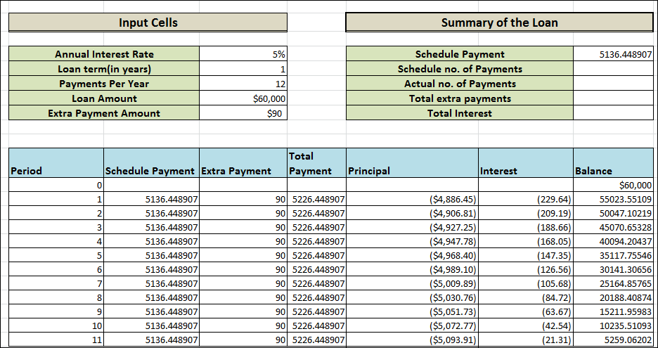
5. Hide Additional PeriodsUtilise this tip to set up the conditional formatting rule that hides values in unused periods. The distinction is that this time, we fill the rows with zero or empty values for Balance (column H) and Total Payment (column E) by using the white font colour: =AND(OR($E12=0, $E12=""), OR($H12=0, $H12=""))
And just like that, no rows using zero values are visible. To conceal zero values in extra periods, implement a conditional formatting rule. 6. Write a Summary of the loanTo add the final touch for perfection, you can use the following formulas to produce the most crucial details about a loan: Scheduled No. of Payments: The number of years multiplied by the annual payment amount is: =Loan Term*Payments Per Year
Actual No. of payments: Count the cells that are larger than zero in the Total Payment column, starting with Period 1: =COUNTIF(E13:E24,">"&0)
The total amount of additional/Extra payments: Start with Period 1 and add up the cells in the Extra Payment column. =SUM(D13:D24)
Total Interest: Start with Period 1 and add up the cells in the Interest column. =SUM(G13:G24)
Once you hide the row containing Period 0, the loan's amortization schedule, including extra payments, will be completed! The final result is displayed in the screenshot below: 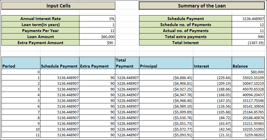
Next TopicCreating a Database in Excel
|
 For Videos Join Our Youtube Channel: Join Now
Feedback
- Send your Feedback to [email protected]
Help Others, Please Share


