How to Calculate ATR in Excel

The average true Range, or ATR, is a term you have undoubtedly heard if you buy stocks or stay informed about commodities markets. This particular type of market indicator highlights a product's price volatility. We'll discuss this in this tutorial and walk you through figuring out the Excel average true range. Without delay let's dive into the concept.

Average True Range(ATR): What Is It?

This method of determining volatility was first presented by Welles Wilder in 1978. An indication of volatility commonly used to describe a stock's price range is the difference between its highest and lowest points on any particular day. That being said, if prices move dramatically on any day, everyone often suspends trading. There is sometimes a discrepancy between the opening & closing prices for two consecutive days when this happens in the commodities trade. Not every day's Range would contain this information. The need for ATR now arises. Within a certain time frame, it shows the average price movement of an asset. Investors may utilise the indicator to choose the best time to trade. Despite being our tool of choice for trend predictions, it cannot predict the direction of price movement. All upcoming contracts, however, are currently tied to the ATR.

Generic Formula for Calculating Average True Range

Calculating an average true range of a stock requires knowledge of its daily close price, daily high, and daily low. We must first be aware of the stock's daily Range. Nothing about it is challenging. In a nutshell, it's the variation in pricing throughout a given day.

If the closing price from yesterday doesn't fall within the daily Range, we need to keep another factor in mind. Afterwards, the true range formula becomes as follows.

In other words, it selects the largest difference between these three options. Stated differently, the true average might be defined as the highest value among the subsequent three.

• The difference between the current high and low
• The current high minus the previous close in absolute terms
• The difference between the current low's absolute value and its previous close

The average true Range of the first period can be computed as follows.

Welles suggested a 14-day smoothed average. Therefore, n = 14 in the formula above. Our initial average true Range will be obtained by first averaging the true Range over the first 14 days. An exponential moving average will then be used to compute the subsequent ATRs. Here, we'll apply the subsequent formula.

ATRt denotes the average true Range in this case.

• ATRt-1 denotes the previous Average True Range.
• Since we're utilising a 14-day moving average, n stands for 14.
• TRt represents the current true Range.

At last, the formula takes on the appearance seen below.

Since ATR exposes the average volatility across the preceding 14 days, and 14 days are regarded to yield the most accurate results, the typical value of n is 14.

Five Steps to Calculate Excel's Average True Range

Assume we are holding a report on "XYZ" Company's stock price. The highs and lows, along with prices of a specific stock from May 25, 2021, to June 23, 2021, are included in this dataset.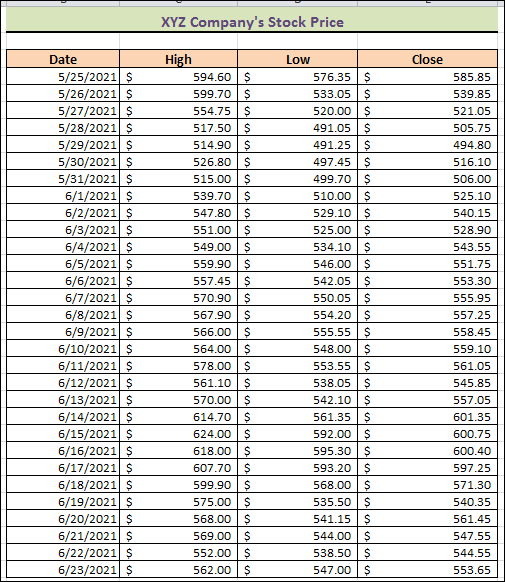

We will now demonstrate how to use this data to get the average true Range in Excel.

Although we've utilised Microsoft Excel 10 here, you're welcome to use any other better version.

Step 1: Calculate the Current High Minus the Current Low

We'll figure out the daily ranges right now. To accomplish this, carefully follow the procedures.

Steps:

1. First, choose cell F4, then type the formula below into that cell.

Here, the corresponding day's high and low prices are denoted by C4 and D4.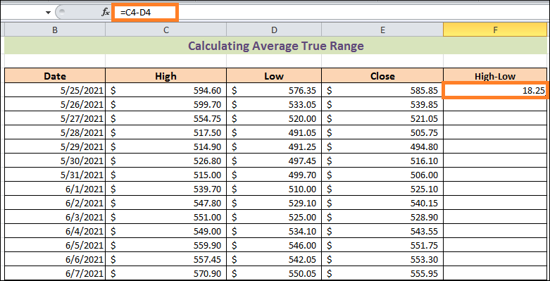

2. Hit the ENTER key a second time.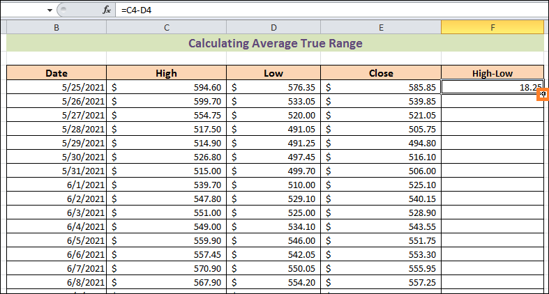

3. Thirdly, the cursor will appear as a plus (+) sign in cell F4's bottom-right corner. The tool is called Fill Handle. Then, to utilise the tool, double-click on it.

Amazingly, it produces the right answers in each subsequent cell up to cell F33. We save so much time by using this tool.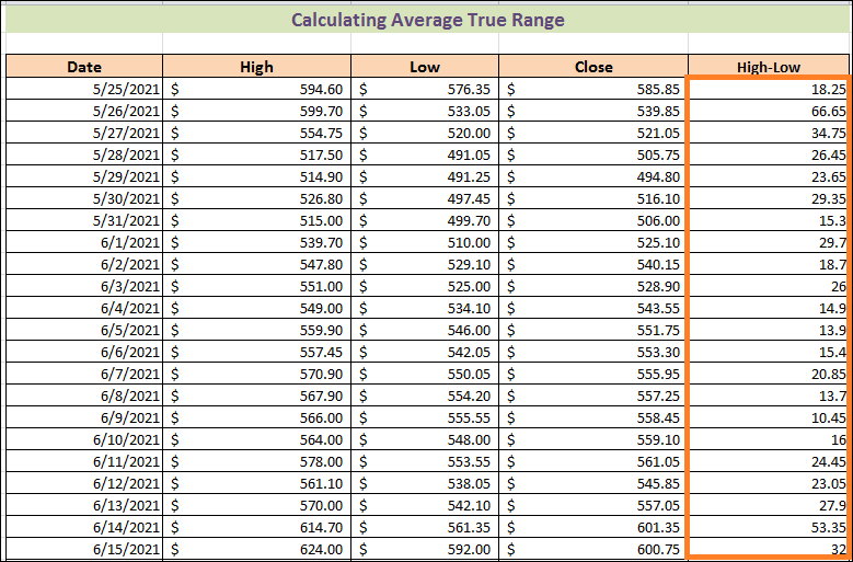

Step 2: Subtract the previous close from the present high

Next, the second component of the above-mentioned true range formula will be computed. Let's see, practically.

Steps:

1. First, choose cell G5 and enter the formula below.

In this case, C5 and E4 are the closing prices from the prior day and the current high price. For each difference, the ABS function yields the absolute value. This indicates that a positive number is always returned.

2. Press ENTER after that.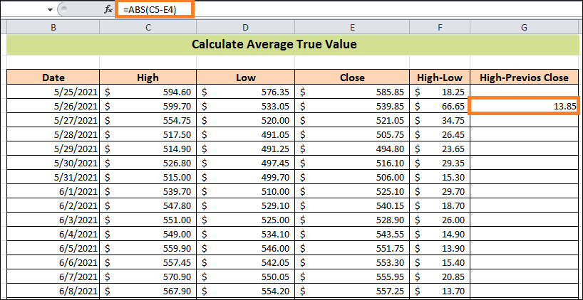

Step 3: Calculate the Current Low Minus the Previous Close

This section will teach the third component of the previously mentioned true range formula. Take a closer look at the procedure.

Steps:

1. It would help if you had first copied the formula below into cell H5.

2. Click ENTER secondarily.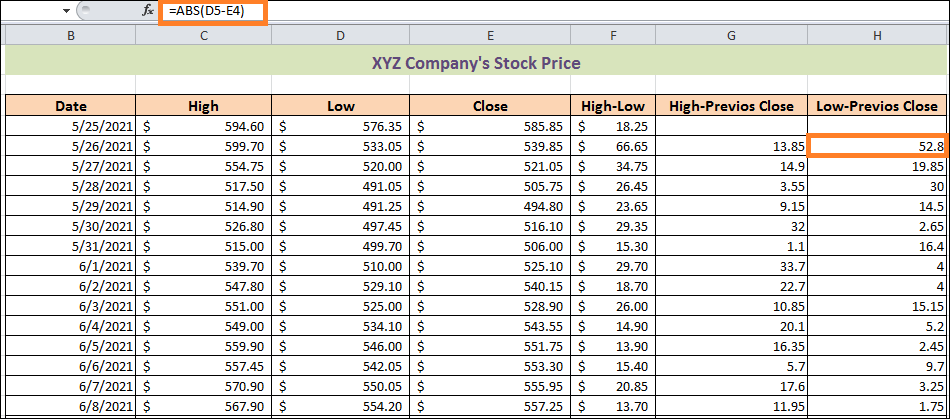

3. There is no day previous to these days; hence, cells G4 & H4 are blank in this instance.

Step 4: Determine the True Range

Now, we'll determine the true Range using the data from the first three phases. Just follow along; it's that straightforward and uncomplicated.

Steps:

1. First, choose cell I5 and enter the below formula in it.

F4:H4 in this formula denotes the cells with high and low, high-previous close, & low-previous close values. In this case, the MAX function returns the data within cells F4, G4, & H4's maximum value.

2. Then, press the ENTER key.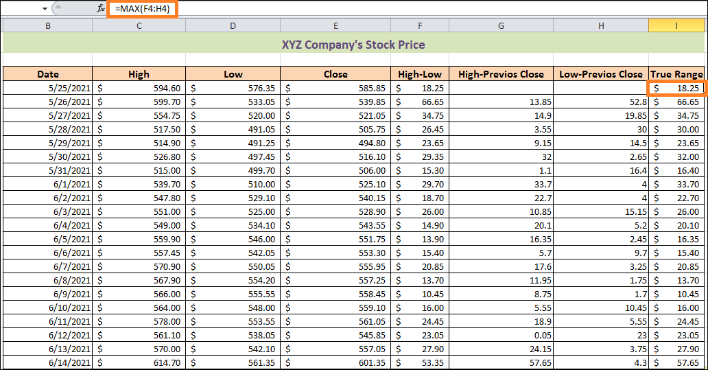

Similarly, we can see if cell I6 yields the right result or not using the formula. In cells F5, G5, & H5, there are 66.65, 13.85, and 52.8. It is evident to us that 66.65 is the most effective of them all. Cell I5 receives the same value from the function as well.

Step 5: Determine the Average True Range

The phase has finally arrived. After finishing this section, we will have the ideal average true Range.

Steps:

1. Choose cell J17 first, then copy and paste the following formula.

The arithmetic mean among the parameters is what the AVERAGE function delivers in this scenario.

2. Press Enter as usual.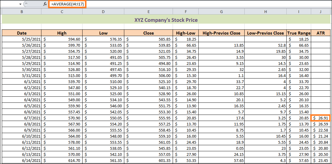

Why are the cells in J4:J16 still blank? Any thoughts? Just return to the general formula we previously covered. There, we said that the average arithmetic value of the next 14 days will be used to compute the ATR of the initial phase. Here, we have utilised data from 14 days in cells within the I4:I17 range.

3. Next, we need to calculate ATR for the days that follow. To accomplish this, input the following formula in cell J18.

In the earlier section, we also went over this formula.

4. Thus, press the ENTER key.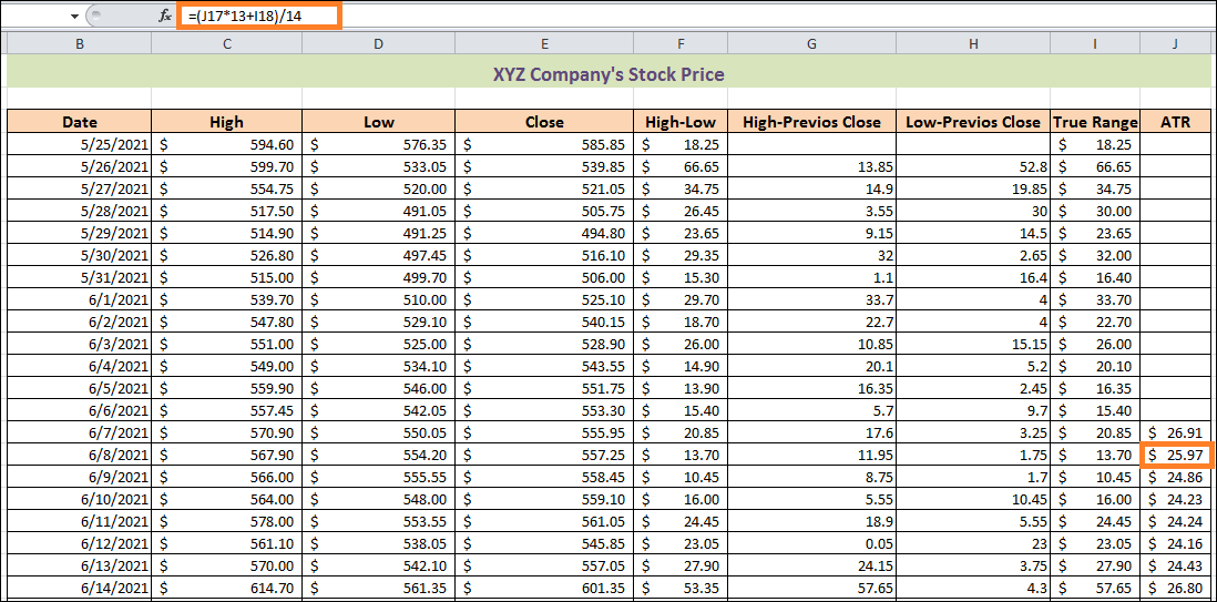

How is ATR Stop Loss Calculated?

We recently learned to use Excel to compute the average true Range. When deciding where to place your stop loss, ATR can help. An appropriately placed stop loss functions as insurance against excessive loss. If you are working with a stock with a high ATR, you should expect wider stop losses because the stock will likely experience more significant daily price movements.

At this stage, you can select the market you're trading according to your risk appetite by multiples based on the ATR reading (2x/3x). The perfect number isn't set in stone. You have to decide based on your past expertise and the industry's current status.

As a general guideline, we chose the ATR value's second multiple. The stop loss on each date will then be determined. Alright, let's get started right now!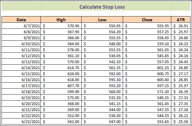

Steps:

1. First, make Stop Loss a new column.

2. Enter the following formula in cell G4 at this point.

3. Hit ENTER after that.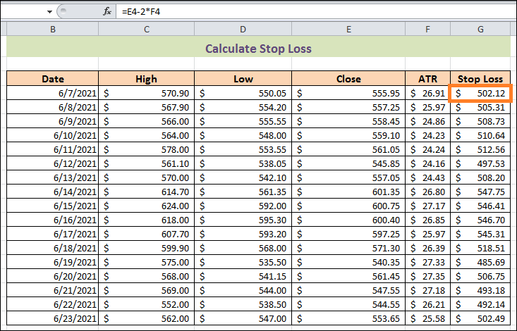

We're going to explain it immediately for clarity. Assume, for example, that on June 7, 2021, you bought shares at its closing price of S555.95. The next step is to establish a stop loss of S502.12. If the stock price drops to that level, you will sell the stock without taking any additional risks.

Likewise, if an investor purchases it on June 18, 2021, at S571.30, he should take the second multiple for the ATR reading and put the stop loss at S518.51.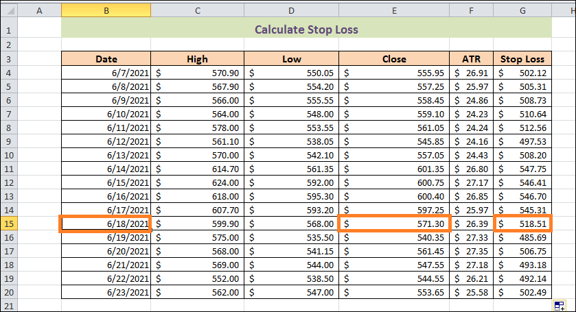

Conclusion:

That's it with this tutorial. By following the given steps, you can easily calculate the Average True Range (ATR) for your data in Microsoft Excel. Make sure to provide accurate data into the stock's price volatility and assist in up-to-date decision-making for dealers and investors.