| |

How to make use of Vlookup with Multiple categories or ValuesIt was well known that, in Microsoft Excel when tasked with the purpose of retrieving out all the multiple matching values that are mainly based upon the specific identifier such as an ID or name, the commonly used "VLOOKUP" function falls short as it can only return the first match found as well. However, there is a simple alternative that primarily does not require any deep Excel formula knowledge, and by just utilizing Excel's filtering as well as the sorting functions, users can efficiently extract all the matching values without the need for complex formulas. However, the process begins by just sorting out the data that are based upon the identifier column and which groups are quite similar to the values altogether, aiding in identifying as well as managing them in an effective manner. Once the data is sorted, we are required to apply the available filters to the identifier column, which allows particular users to display only the rows that match with the desired value, effectively isolating out all the relevant subsets of the data, and with the filtered data visible, users can now easily select. They can copy all the matching values from the given corresponding column. Despite all this, copying out the values is as simple as clicking and dragging the cursor in order to select the desired cells, which are mainly followed by a right-click to get access to the copy command. The copied values can then be pasted into a new location within the worksheet, whether it be a different column, a new worksheet, or even a separate Excel file. This intuitive process thus makes it accessible to users of all skill levels, right from beginners to advanced users. And more often, for those who are facing repetitive tasks, creating a macro offers an automated solution to the Excel user. As the Macros primarily enable the particular users to make record of the series of the actions and can also replay them by just having single click. In spite of all this, we knew that while Microsoft Excel provides powerful functions, such as none other than VLOOKUP, for the efficient analysis of the data, simpler methods like filtering as well as sorting often suffice, especially for the purpose of retrieving multiple matching values. Just by following a few straightforward steps, users can now quickly extract the desired data without the need for complex formulas, thus making the data more accessible to everyone. What is the syntax for the Vlookup Function in Microsoft Excel?The syntax of the VLOOKUP Function that can be efficiently used by an individual in an Excel sheet is as follows: 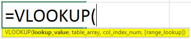
Here, in this particular syntax, the function usually accepts four basic arguments that are none other than the following ones:
Moreover, in the above syntax the very first three arguments are considered as the mandatory one, while the last one is termed to be an optional one as well. So now let us deep dive into this arguments to get more factual information respectively:
How can one make use of the Vlookup with the Multiple Criteria?While making use of the VLOOKUP function in Microsoft Excel, if it locates a matching value in the given specified range, then it case it would stop searching as well as returning the corresponding result, even if there are multiple matches within the given set of the data. Example 1: Vlookup with the multiple matches, and then it will return results in a specific column. Let us assume that we have the names of the sellers in column A, as well as product names that have been sold, represented in column B. Column A contains a few occurrences of each seller as well. Here in this example, our main motive is to just get a list of all the products that has been efficiently sold by the particular person. And to have it done, we are required to follow the below-mentioned steps: 1. First of all, we are required to enter a list of the unique names in some of the empty rows in the same or another worksheet as well. So, in this particular example, the names are mainly inputted in the cells D2:G2: 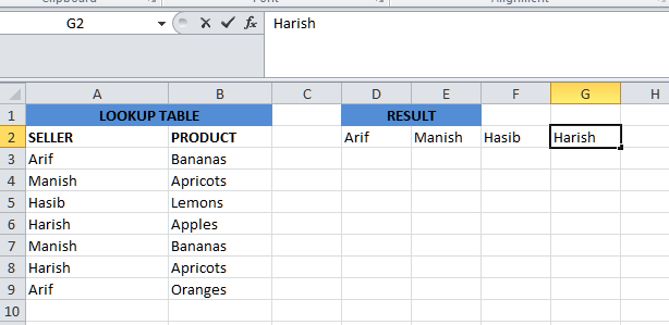
Important note: In order to quickly get all the different names in a list, we can easily make use of the UNIQUE function in Microsoft Excel 365 or a more complex formula for the purpose of extracting the distinct values in the older versions.2. And under the first name, we must need to select out a number of the blank cells which is very much equal to or greater than the maximum number of the possible matches as well, just after that we must need to enter out one of the following array formulas in the respective formula bar, then proceeding with the pressing of the shortcut button that is none other than Ctrl + Shift + Enter, to complete it (in this case, we will be able to edit out the formula only in the entire range where it is entered). Or As we can see, then the 1st formula is more compact, but the 2nd one is more universal, and it requires fewer modifications (we will be elaborating more on the syntax as well as logic a bit further). 3. Now in this step, we are required to copy down all the selected formulas to the other columns. Now, for this particular part, we are about select out the range of the cells in which we actually need to enter out the formula, after that we must need to drag out the fill handle (it is mainly a small square shape box present at the lower right-hand corner of the selected range) to the right respectively. And just after applying out the above mentioned steps, we will be encountered with the output as follows below: 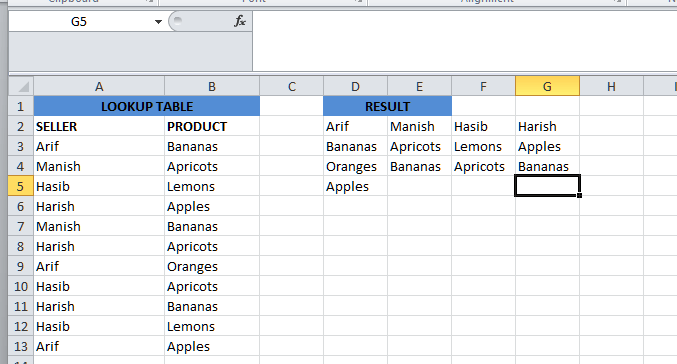
How does this particular formula work? It is well known that it was mainly an example of the intermediate to the advanced uses of Microsoft Excel that primarily determines out the basic knowledge of the array formulas as well as the various functions which are available in the Microsoft Excel. Working from the inside out, here's what we actually do:
More often, at the core of the formula, we can eventually make use of the IF function to get the positions of all the occurrences of the lookup value in the lookup range as well: IF(D$2=$A$3:$A$13, ROW($B$3:$B$13)-2,"") IF Function in this part compares out the lookup value in the cell (D2) with each value in the lookup range that mainly ranges from the cell A3:A13, and if the match is found, then in that particular scenario, it will be returning out the relative position of the row; as an empty string ("") otherwise effectively. However, the relative positions of the rows are calculated by just subtracting 2 from the ROW ($B$3:$B$13) so that the first row has the position 1. If our return range begins in row 2, then we must need to subtract out 1, and then we must need to move on. And the result of this operation is the array {1;2;3;4;5;6;7;8;9;10;11}, which goes to the value_if_true argument of the IF function. Instead of the above calculation, we can now make use of this expression: ROW(lookup column)- MIN(ROW(lookup_column))+1, which returns the same result, but it does not require any changes regardless of the return column location. In this particular example, it'd be ROW ($A$3:$A$13)- MIN(ROW($A$3:$A$13))+1. Now, at this point, we need to have an array that mainly consists of the numbers (positions of the matches) as well as the empty strings (with the position having non-matches). For cell D3 in this example, we have the following array which is as follows: 
Now, if in case we check with the source data, we will see that "Adam" (lookup value in cell D2) mainly appears on the 3rd, 8th, and 10th positions in the lookup range that ranges from (A3:A13), respectively.
Next, the respective SMALL (array, k) function steps are mainly used for the purpose of determining which of the matches should be returned in a specific cell. With the array, which is already been established, so let us now work out with the k argument which is considered as the smallest value and that's need is to be returned out. To achieve this effectively, we can now easily make use of an "incremental counter" ROW ()-n, in which "n" is the termed to be row number of the first formula cell minus 1. Despite of all this, in this particular example, we have now entered out the formula in the cells D3:D7, so ROW ()-2 returns "1" for the cell D3 (row 3 minus 2), "2" for the cell D4 (row 4 minus 2), etc. And as an output, the SMALL function usually pulls out the 1st smallest element of the array in cell D3, while the 2nd smallest element in the cell D4, and so on. This will now transform out the initial long as well as the complex formula into a very simple one, like the below one: 
Important Note: Now, in order to see the calculated value that mainly lies behind a certain part of the formula, we need to select that particular part in the mentioned formula bar, and then after that, we just need to press the function button that is none other than F9 from our respective keyboard.
Note. The proper use of the absolute as well as the relative cell references in the formula should be noticed. And all the references are mainly fixed except for the relative column reference in the lookup value which must need to need to be changed on the basis of the number of the presence of the relative positions of a column(s).# Example 2: Use of Vlookup with the Multiple Values For this particular example, let us assume that we have data on the employees of our respective company that is none other than "GURUKUL." The data contains the "Name," "Current Salary," "Department," as well as the "ID," as it was depicted in the below-mentioned image respectively. 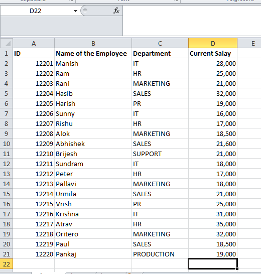
And here in this we primarily want to look up an employee by their specific name and also with the respective department. Despite all this, the particular search will include two details that are none other than the: "Name" and also the "Department." The name and the department to look up are given in cells, which are G6 and G7. 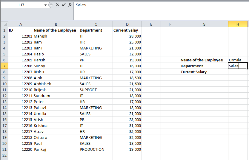
And now if we want to search for the employee whose name is "Urmila" who's working in the "Sales" Department so, to achieve this first of all, we are required to make a separate column which contains the "Name" as well as the "Department" of all the employees who all are working in the respective company. And to do this for the first employee, we can now make use of the Excel VLOOKUP Formula: = C2 & D2. 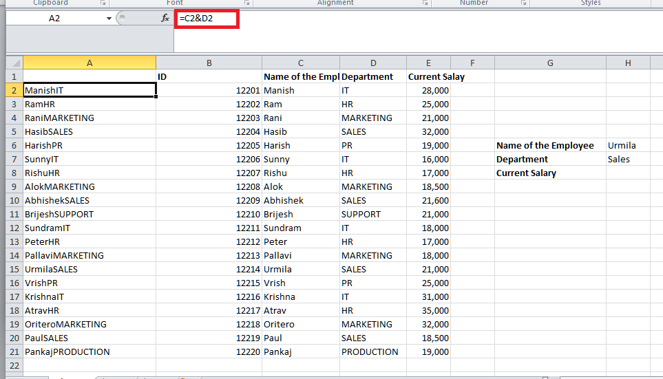
Now, just after that, we need to press the "Enter" key from our keyboard. The cell will now contain "Manish IT." It is very important to add this column to the very left of the data since the first column of the array range is considered for the lookup. Now, we need to drag it to the rest of the cells in an effective manner. 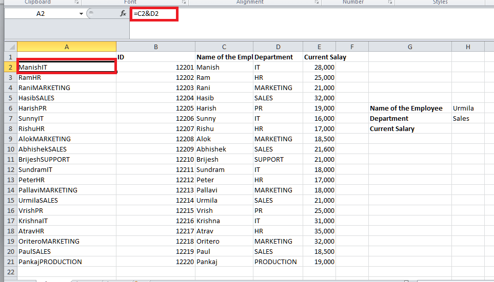
In order to look up the value for the employee "Urmila" and "Sales" given in cells G6 and G7, then in that case we now make use of the Microsoft Excel VLOOKUP formula: = VLOOKUP (H6 & H7, A2:E21, 5, FALSE) 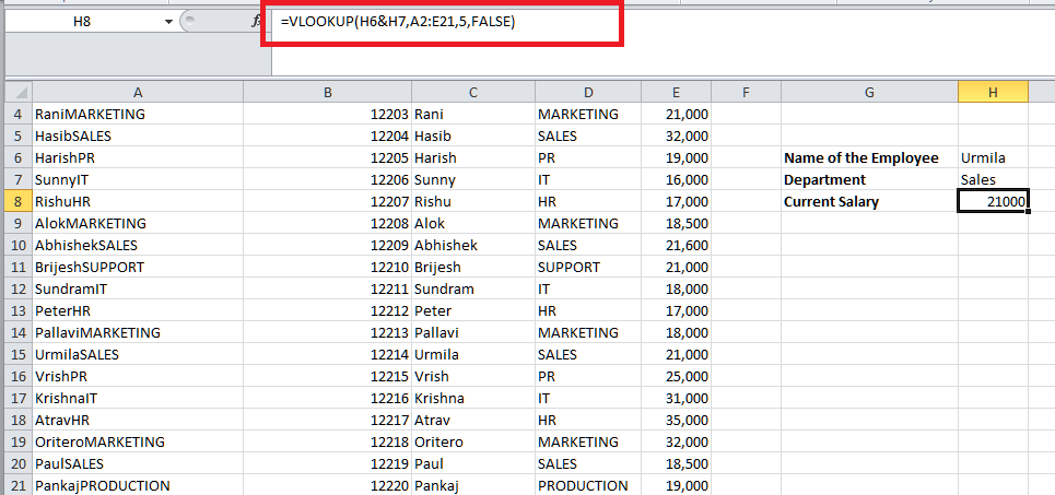
It will now be returning the salary of the lookup employee, Urmila, from the sales department respectively. 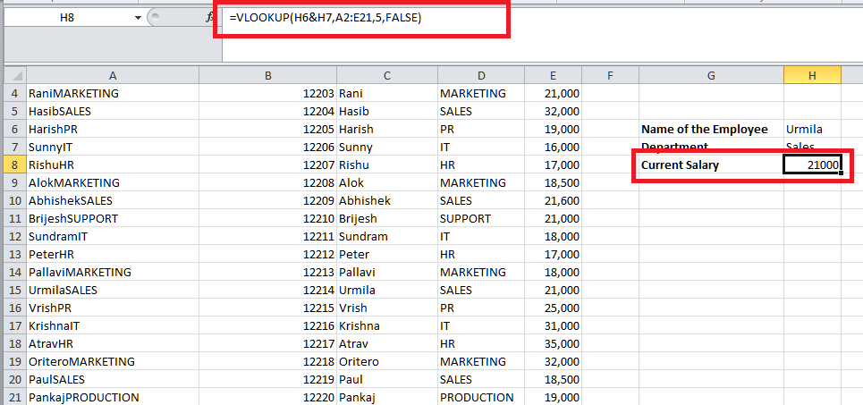
# Example 3: Let us now suppose that we have the data related to the sales and that too for the two different items that have been purchased in the last 12 months, as it was clearly depicted in the below-mentioned table below: 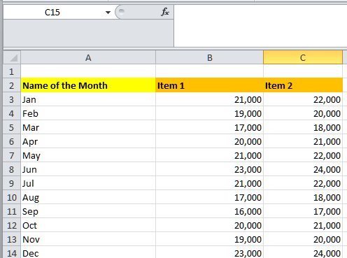
In this, we actually want to create a lookup table in Excel, in which we must enter out the "Month" as well as the "ID of the Item" (item 1 and item 2 in this case), which will then be returning out the sales for that particular product during that specific month respectively. 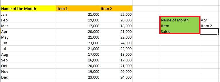
To achieve this easily, we now make use of the VLOOKUP as well as the Match Formula in Excel: = VLOOKUP (F4, A3:C14, MATCH (F5, A2:C2, 0), 0) More often, the month that we want to look up is mainly encountered in cell F4, as well as the item name to look for is in cell F5 effectively. 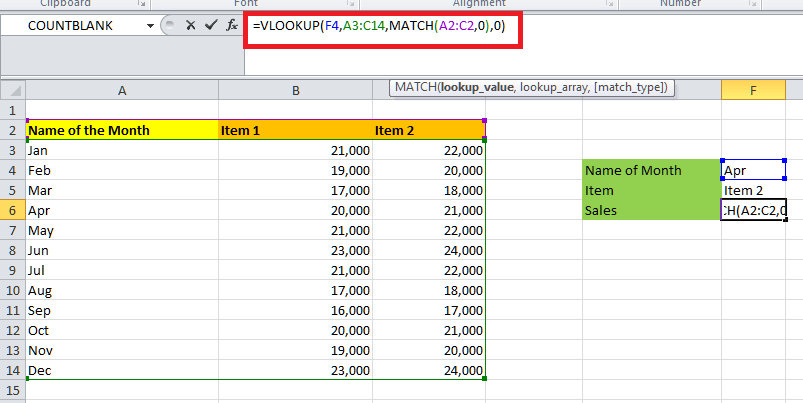
And in this particular example we will be getting the output as 21,000. 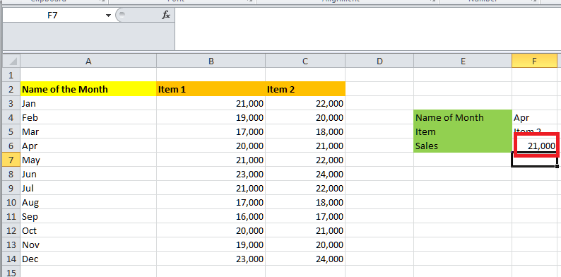
# Example 4: In this example, let us suppose that we have the data related to the sales that have been collected for one of the products that have been sold out throughout the year in four different city zones. The table for this data has been depicted in the below-mentioned image as well. 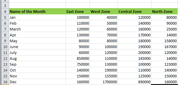
Now, if in case we actually want to check if the month in which the sales were quite maximum for the "East Zone" is also the month in which sales were maximum for the "West Zone." In order to check this, first of all, we are required to make use of an additional column that contains the sales for the east as well as for the west zone. Here, in this case, we would like to separate the values with the help of the <space> button from our respective keyboard. In spite of all this, if in case we want to add the additional column to the left-hand side of the sheet, then we can make use of the Excel VLOOKUP formula: = D3 & ""& E3. 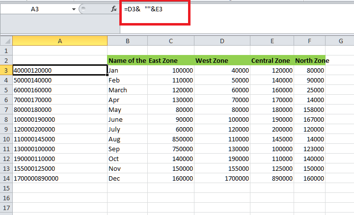
For the table's first cell, we are required to press the "Enter" key from our respective keyboards. Then, after that, we need to drag it to the rest of the cells efficiently. 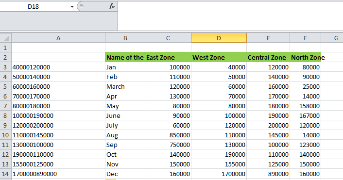
After that, we are required to calculate the maximum sales for "East Zone" and "West Zone" separately. For the purpose of calculating the maximum value, we can now make use of the Excel VLOOKUP formula as well: = MAX (D3:D14) for East zone 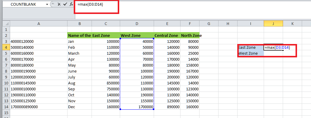
= MAX(E3:E14) for West Zone respectively. 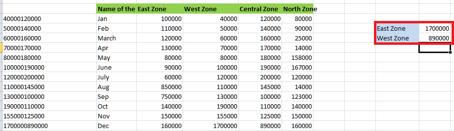
Now, if in case we want to check if the month for which sales were maximum for the "East Zone" is also the month in which sales were quite maximum for the "West Zone," also and for this, we can easily make use of the following formula: = IFERROR (VLOOKUP ( J4 &" " & J5, B3:C14, 2, 0), "NO") 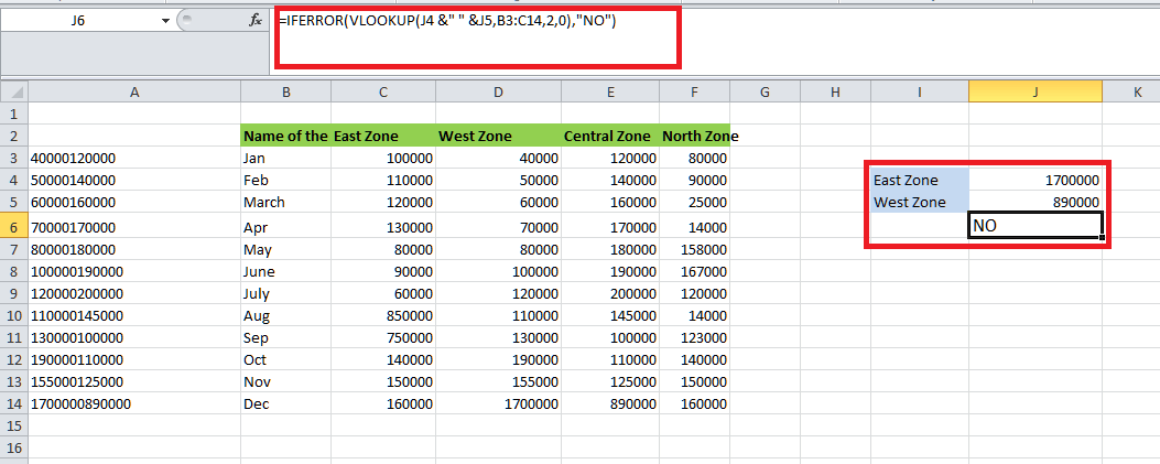
VLOOKUP ( J4 &" & J5, B3:C14, 2, 0) will now automatically search for the maximum "East Zone" and the "West Zone" values in the additional column. If it can find a match, then it will be returning out the corresponding month as well. Else, it will give an error. IFERROR ((VLOOKUP(..)), "NO"): If the output from the VLOOKUP function is an error, it will return "NO" else. It will return the corresponding month. Since no such month exists, let us check if the month in which the sales were maximum for the "East Zone" is the month in which the sales were second-highest for the "West Zone." First, calculate the second-largest sales for the "West Zone" by using: = LARGE(E3:E14, 2) 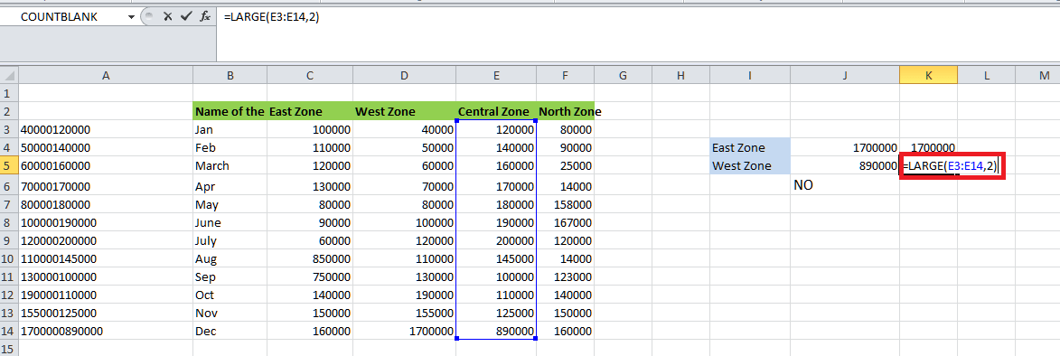
Now, use the syntax: =IFERROR (VLOOKUP(K4&" "&K5, B3:C14, 2, 0), "NO"). 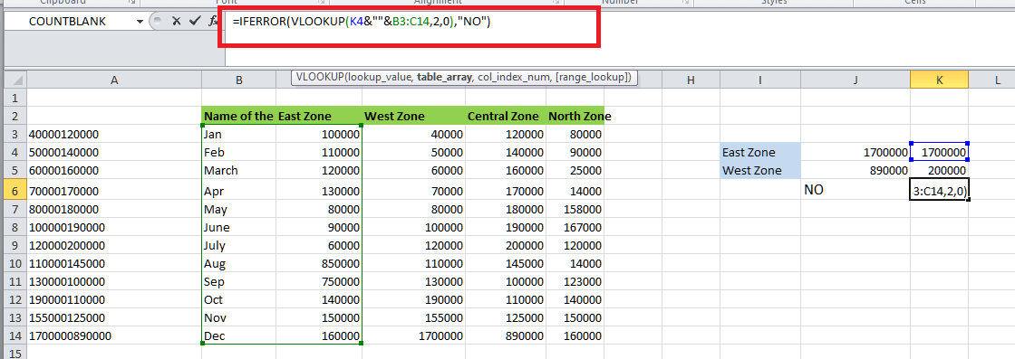
It will return "June." 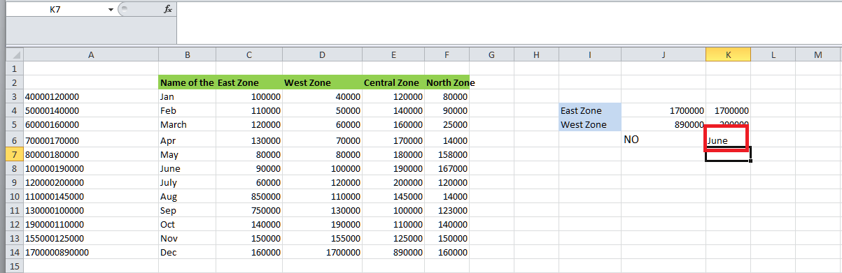
It is very important to note that there can be more than one month in which the respective sales were quite maximum for the "East Zone" and "West Zone," but the Excel VLOOKUP formula will only return one of those months. List out the advantages of using VLOOKUP with the Multiple Criteria or Values in Microsoft Excel.It was well known that making use of the respective VLOOKUP with the multiple criteria or values mainly offers various significant advantages that can greatly enhance our management of the data and its analysis tasks. So let us now break down all these benefits in simpler terms respectively: 1. Increased Rate of Accuracy: The VLOOKUP is like a searching tool. And when we are searching for the data online, the more specific our search terms, the more accurate our results will be as well. In the same way, by just making use of the multiple criteria in the VLOOKUP, here we are providing some more detailed instructions on what we are actually looking for. This will help us to reduce the chances of getting incorrect as well as irrelevant information back. 2. Flexibility of Searching Data: Let us imagine that we are searching for a specific item in a store, but we are not just looking for any item; we want one that eventually meets certain criteria, such being a certain kind of color as well as the size. The respective VLOOKUP function with the multiple criteria works similarly. And despite this, it allows us to specify exactly what we are looking for by combining different conditions. So, you can find data points that match various requirements, even if they are spread across different columns or in different categories. 3. Dynamic Retrieval of the data: Now have you ever had to redo a specific search it is because of the reason that our initial criteria may have been changed slightly? And with the VLOOKUP and multiple criteria, one can easily avoid that type of hassle. More often, this particular feature helps us set up our particular search in order to adapt to the changes automatically. So, if in case our requirements evolve or our respective dataset gets updated, our VLOOKUP formulas can still find the right information without needing manual adjustments every time as well. 4. Efficiency: It is well known that searching through a massive dataset manually is like looking for a needle in a haystack, and it is quite time-consuming and also exhausting. VLOOKUP with the multiple criteria is just like having a supercharged search engine that can sift through the haystack in seconds and can now pull out exactly what we actually need. This will save us a ton of time as well as effort, thus allowing us to focus on the other important tasks effectively. 5. Enhanced Analysis: In some cases, we are required to dig deeper into our data for the purpose of uncovering insights or trends. And for that particular case the respective VLOOKUP with the multiple criteria or the values can gives us power to complete the task effectively, inspite of this we can also make cross-reference to the various conditions for the purpose of performing out more sophisticated analyses, as It is was bit like having a magnifying glass for our selected data, that in turns allows us to zoom in on the specific patterns which might otherwise go unnoticed. However, effective use of the VLOOKUP function with the multiple criteria is more about like having a versatile and as an efficient assistant for the tasks in correlation with the data, and it wills also helps us to find out the right information quickly and in an accurate manner, adapt to changes seamlessly, and also to uncover out the valuable insights that can inform our decision-making process. List out the disadvantages of using VLOOKUP with the Multiple Criteria or Values in Microsoft Excel?The various disadvantages of using VLOOKUP with the Multiple Criteria or values in Microsoft Excel are as follows:
Next TopicHOW TO RESIZE CELLS IN EXCEL
|
 For Videos Join Our Youtube Channel: Join Now
Feedback
- Send your Feedback to [email protected]
Help Others, Please Share


