| |

Recurring Deposit in ExcelYou've arrived at the correct place if you've been searching for some unique tips on how to use Excel to compute compound interest for recurring deposits. In this detailed tutorial, will show how to use Excel to compute compound interest, or the maturity value, for recurring deposits. It will be difficult to save money if your budget is loose. But there are numerous reasons why saving is crucial in life. Our goal is to preserve:
Certain people find saving difficult. For those that fit this description, setting up a monthly automatic payment into their savings finances and receiving a sizable payout after a few years is wise. In the Indian subcontinent, recurring deposits, or RDs, are a common savings plan. Recurring Deposits (RDs) are well-liked for the reasons listed below:
Now, allow me to demonstrate how to use Excel to determine a recurring deposit's compound interest (maturity value). Understanding how everything functions for your investment is a good habit. Regarding your finances, you should never be left in the dark. Excel Functions We'll Use to Compute Compound Interest on Recurring DepositsExcel has significantly eased our life. Using the FV function, you may quickly determine your recurring deposit's Maturity Value (Future Value) at any time. When you make monthly deposits, things get complicated, and the bank multiplies your funds every quarter or at different times. Be at ease. I am going to simplify things for you. We will walk you through the entire calculation step-by-step. We'll utilise a few Excel functions here: 1. FV FunctionThe FV function yields the future value of an investment, which is based on regular, fixed payments & a constant interest rate. The FV function's syntax: FV(type, pv, pmt, nper, rate)
In this,
2. EFFECT FunctionThe EFFECT function returns the annual effective interest rate. EFFECT Function Syntax: EFFECT (nominal_rate, napery)
In this,
Take your bank's 5% annual Nominal Interest Rate, for instance. When you deposit $500 with a bank, the bank will compound your money every quarter for the following year. Which effective rate of return will you get? It is 1.25%, or 5%/4, as your rate per quarter. The reason for this is that your funds are compounded four times annually. The nominal interest has been divided by 4 to obtain the Rate per Quarter. Look at the picture down below: 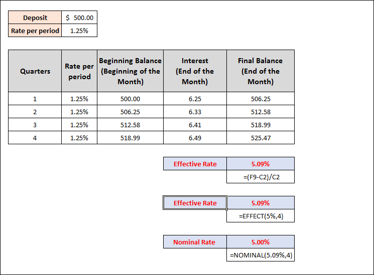
You observe that:
It is a 5% nominal interest rate for you. However, you're receiving a 5.09% return on your investment because of the four compoundings that occur each year. The Effective Rate shown above can be obtained by using the EFFECT function within cell F14: =EFFECT(5%, 4)
Additionally, this is also there in the image. 3. Nominal FunctionComparable to the EFFECT function is the NOMINAL function. An Effective Interest Rate is used to calculate the Nominal Interest Rate. Syntax of the nominal function: Nominal (effect_rate, napery)
The Nominal Interest Rate is obtained via an Effective Interest Rate using this function, which is utilised in cell F16. =NOMINAL(5.09%,4)
Two Simple Ways to Compute Compound Interest on Recurring Deposits in ExcelIn the next section, we'll calculate compound interest on recurring deposits in Excel using two efficient yet challenging methods. The FV function will be used in the first approach and the direct way in the second. You should study and use these to increase your capacity to think critically and your familiarity with Excel. We're using Microsoft Word 2010, but you can use any other version that suits your needs. 1. Making Use of the FV FunctionHere, we'll walk you through how to use Excel to compute compound interest on regular deposits. We'll start by introducing our Excel dataset so you can better understand our goals for this essay. The FV, EFFECT, NOMINAL, & VLOOKUP functions will all be used in this procedure.
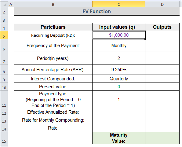
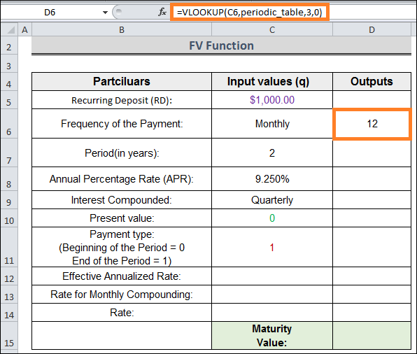
The following procedures will demonstrate how to use Excel to determine recurrent deposits' compound interest (also known as the maturity value). Procedure:
= VLOOKUP(C6, periodic_table, 3,0)
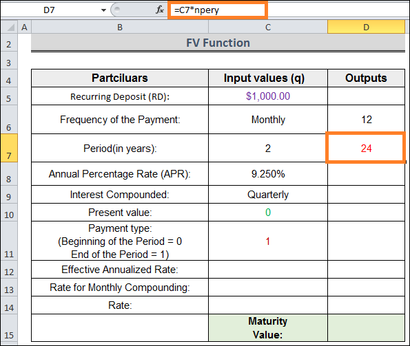
= C7*npery
=VLOOKUP(C9,periodic_table, 3,0)
Remember that the Interest Compounding Frequency should match or exceed the Payment Frequency. For instance, you cannot select weekly, bi-weekly, or semi-monthly as your compounding frequency if the payment frequency is monthly. 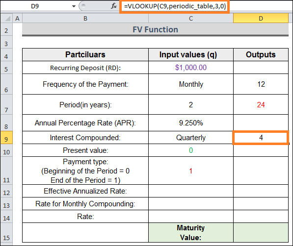
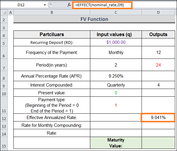
= EFFECT(nominal_rate,D9)
=NOMINAL(D12, napery)
*Note: Here's a technique to double-check if monthly compounding would result in the same effective rate as this nominal rate (8.687%): =EFFECT(8.687%,12) =9. 041% Same.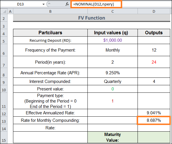
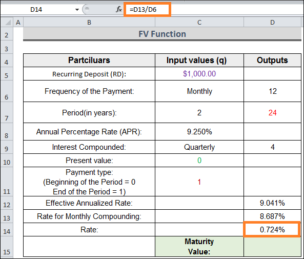
= D13 / D6
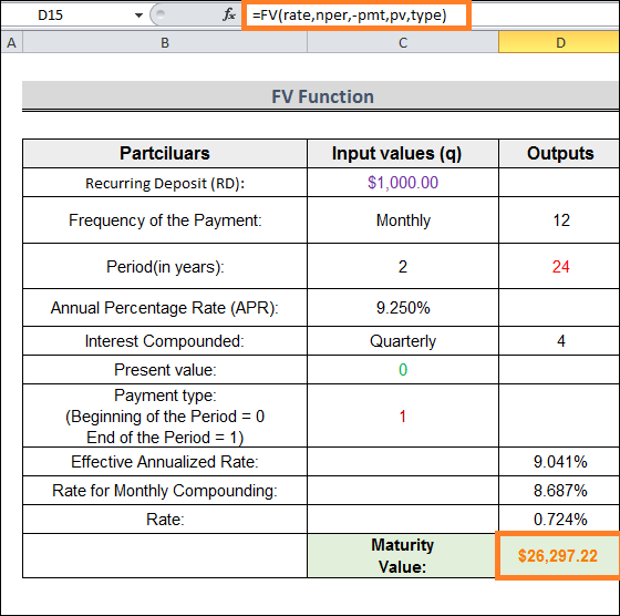
=FV(rate,nper,-pmt,pv,type)
The procedure we used to determine the repeating deposit is depicted in the below image. 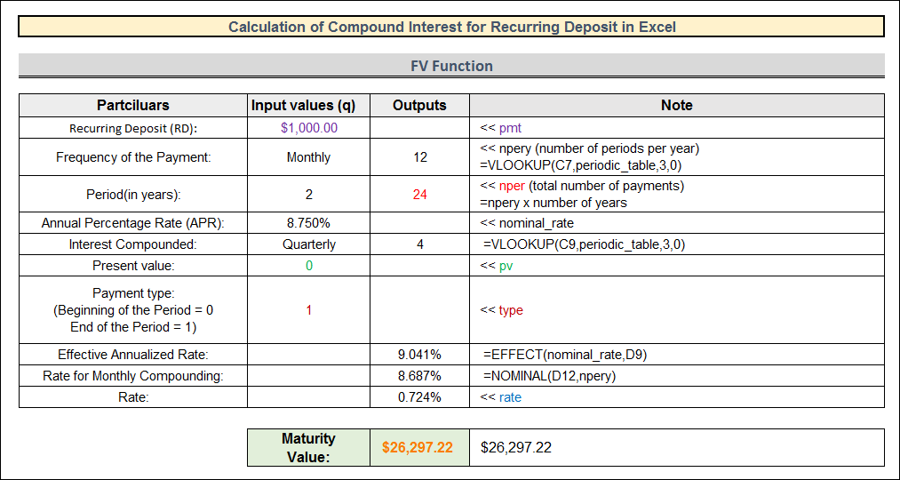
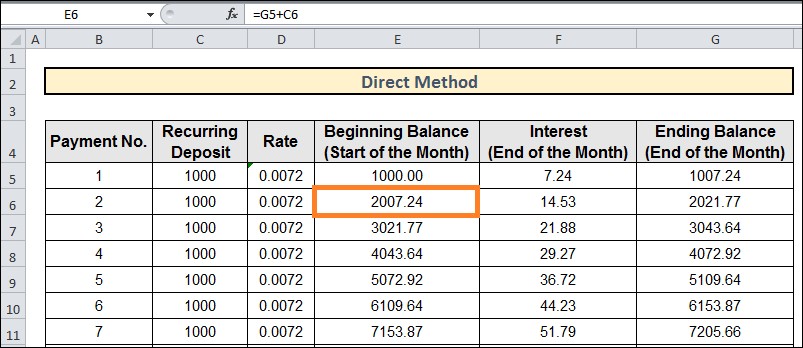
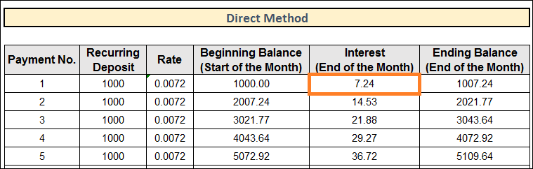
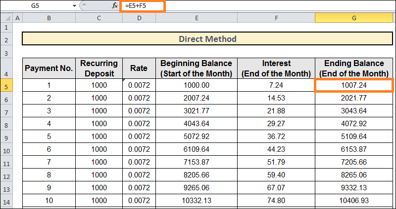
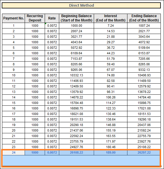
2. Using the Direct MethodThis methodical computation determines your Recurring Deposit's (RD) Maturity Value over 24 periods (Two years). Here, we've applied identical PMT values and period-wise rates. But the process is straightforward. View the graphic below for a breakdown of our steps to determine the recurring deposit using the direct technique. 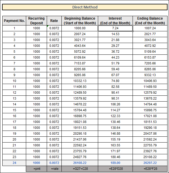
Let's clarify. Let's go over how to compute the recurring deposit in the following steps. Procedure:
G5 + C6
= E5 * D5
= E5+F5
Next TopicTDS Calculator in Excel
|
 For Videos Join Our Youtube Channel: Join Now
Feedback
- Send your Feedback to [email protected]
Help Others, Please Share


