Automated Trading in Python

Because Python accelerates the trading process, this method is known as automated or quantitative trading. Python's popularity is due to its powerful libraries, like Pyplot, TA-Lib, Scipy, NumPy, Zipline, Matplotlib, Pandas, etc.

What is Automated Trading?

Automated trading engages capital markets by executing pre-set procedures for accepting and leaving trades using a computer program. As a trader, one will combine in-depth statistical analysis with the creation of position characteristics like open orders, guaranteed stops and trailing stops.

Auto trading allows us to make a large number of deals in a short period while also removing emotion from our investment choices. This is true because our constraints already include all of the trading rules. We can even utilize our pre-determined techniques to monitor trends and trade correspondingly to some algorithms.

How does Automated Trading Work?

We'll start by selecting a platform and defining the characteristics of our trading plan. We'll construct a set of terms and regulations based on our trading expertise, and our bespoke algorithm will use the information to conduct bets on our account. The scheduling of the deal, the cost at which it must be opened or closed, and the number are usually the determining considerations. 'Buy 100 Google shares whenever the 100-day moving average crosses the 250-day moving average,' for example.

The established automated trading method will continuously watch financial market rates, and deals will be completed automatically if predefined conditions are reached. The goal is to conduct transactions more quickly and efficiently and profit from technical market happenings.

Benefits of Automated Systems

There are a lot of benefits to letting a computer watch the marketplace for trading activities and conduct the trades, including:

Emotional Control

During the buying and selling, automated trading systems reduce sentiments. By holding emotions under control, traders often have a better time adhering to the trading plan. Traders could not pause or challenge the trade because trade instructions are performed automatically when the trade regulations are met.

Backtesting

Backtesting determines the feasibility of a concept by applying trade laws to previous market data. When building a framework for automated trading, all rules must be precise, with no room for ambiguity. The machine cannot make educated guesses and must be given specific instructions. Traders can use past data to evaluate these specific rules before risking capital in trading.

Maintaining Discipline

Even in volatile times, discipline is maintained since market rules are formed, and trade operation is executed automatically. Emotional considerations such as being afraid of losing money or the urge to squeeze a bit more revenue out of a deal cause focus to be lost. Since the computer will carry out the trading strategy exactly as formed, automated trading aids in retaining discipline.

Increasing the Speed of Order Entry

Automated systems can produce bids as quickly as trade conditions are satisfied since computer systems react quickly to fluctuating market situations.

Trading Diversification

Trading numerous portfolios or tactics at once is possible with automated trading systems. This can disperse risk across multiple instruments while providing a buffer against losing trades.

Necessary Elements for Automated Trading

Anaconda: The first task in installing Python is to install Anaconda. Anaconda is a dependable Python platform that includes all utilities and modules needed to run Python programming.
Spyder IDE: IDE is the short form of Integrated Development Environment. It provides a user interface for writing, debugging, compiling, and running Python programs.
Jupyter Notebook: Jupyter Notebook provides an interactive environment for debugging programs. Jupyter Notebook principally employs 'markdown' cells for code explanations and 'code' cells for executing the code. It's very helpful for students attempting to figure out how code snippets function.

Useful Packages/ Libraries in Python for Automated Trading

Python has a major resource of libraries that we may use for various purposes like coding, machine learning, visualization, etc. We'll have to import financial information, do a numerical analysis, create trading strategies, draw graphs, and backtest data. The following libraries are required:

NumPy (short for NumericalPy) is a Python package for numerical data processing.
When dealing with datasets in a tabular format (i.e., rows and columns), like spreadsheets, Pandas is extensively employed. We can use it in Python programming to load Excel and CSV files.
Matplotlib library contains a method for plotting two-dimensional graphs.
TA-Lib is a popular tool for performing a technical evaluation of data like Bollinger Bands, RSI, VWAP, and MA (Moving Average).
An event-driven platform with backtesting and real-time trading capabilities.

Setting Up Work Environment

Installing Anaconda is the quickest way to get started with automated trading. The Python package Anaconda includes a variety of IDEs, including Spyder, Jupyter, __, ___, libraries for analysis, etc.

Installing the Yahoo-Finance Module

We can retrieve the stock's previous data with the help of the Yahoo Finance module. Type the following command line in the terminal and hit enter to install Yahoo Finance:

Code

Importing the Required Packages

The following step after installing yfinance is to import packages in our program to run trading algorithms. Due to the extensive data modification required for backtesting, we will use Pandas strictly throughout this course.

Code

import pandas as pd
import yfinance as yf

Getting Stock Financial Information

Financial data retrieval is also incredibly simple in yfinance. Simply use the company's ticker as an argument for the ticker function. The code below uses Tesla shares as an illustration:

Code

# Python program to show how to get info of any stocks using Ticker method of yfinance

# Importing the required module
import yfinance as yf

# Retrieving data using Ticker
Tesla = yf.Ticker("TSLA")

# Printing the Tesla stocks info:- it is a dictionary
print(Tesla.info) 

Output:

{'zip': '78725', 'sector': 'Consumer Cyclical', 'fullTimeEmployees': 99290, 'longBusinessSummary': 'Tesla, Inc. designs, develops, manufactures, leases, and sells electric vehicles, and energy generation and storage systems in the United States, China, and internationally? The company was formerly known as Tesla Motors, Inc. and changed its name to Tesla, Inc. in February 2017. Tesla, Inc. was incorporated in 2003 and is headquartered in Austin, Texas.', 'city': 'Austin', 'phone': '(512) 516-8177', 'state': 'TX', 'country': 'United States', 'companyOfficers': [], 'website': 'https://www.tesla.com', 'maxAge': 1, 'address1': '13101 Tesla Road', 'industry': 'Auto Manufacturers', 'ebitdaMargins': 0.20424, 'profitMargins': 0.13505, 'grossMargins': 0.27096, 'operatingCashflow': 13850999808, 'revenueGrowth': 0.805, 'operatingMargins': 0.1549, 'ebitda': 12702000128, 'targetLowPrice': 67, 'recommendationKey': 'buy', 'grossProfits': 13606000000, 'freeCashflow': 7054624768,...}

The print statement produces a Python dictionary, which we can use in analysis by getting the specific financial data we're looking for from Yahoo Finance. Let's take a few fiscal critical metrics as an example.

The info dictionary contains all firm information. As a result, we may extract the desired elements from the dictionary by parsing it:

Code

# Python program to show how to access data from the info of shares
print(Tesla.info['shortRatio']) 

print(Tesla.info['regularMarketDayHigh'])

print(Tesla.info['marketCap'])

Output:

0.85
759.19
728613322752

There is a tonne of more stuff in the info dictionary. By printing the info keys, we can view all of them:

Code

# Python program to show how to print keys of the info dictionary

print(Tesla.info.keys())

Output:

dict_keys(['zip', 'sector', 'fullTimeEmployees', 'longBusinessSummary', 'city', 'phone', 'state', 'country', 'companyOfficers', 'website', 'maxAge', 'address1', 'industry', 'ebitdaMargins', 'profitMargins', 'grossMargins', 'operatingCashflow', 'revenueGrowth', 'operatingMargins', 'ebitda', 'targetLowPrice', 'recommendationKey', 'grossProfits', 'freeCashflow', 'targetMedianPrice', 'currentPrice', 'earningsGrowth', 'currentRatio', 'returnOnAssets',?)

Retrieving Historical Market Prices

Continuing with other resources the yf library has to offer. Additionally, we can utilise it to get market data from previous years.

We will use historical Tesla stock prices in the example below over the past few years. It is a relatively easy assignment to complete, as demonstrated below:

Code

# Python program to show how to get historical stock prices of a stock

# Importing pandas to create a dataframe
import pandas as pd

# Getting historical stock prices when price was maximum
prices = Tesla.history(period="max")

# Creating a data frame of prices
df = pd.DataFrame(prices)

# Printing the head of the data frame
print(df.head())

Output:

             Open   High    Low  Close    Volume  Dividends  Stock Splits
Date                                                                     
2010-06-29  3.800  5.000  3.508  4.778  93831500          0           0.0
2010-06-30  5.158  6.084  4.660  4.766  85935500          0           0.0
2010-07-01  5.000  5.184  4.054  4.392  41094000          0           0.0
2010-07-02  4.600  4.620  3.742  3.840  25699000          0           0.0
2010-07-06  4.000  4.000  3.166  3.222  34334500          0           0.0

We obtained the maximum quantity of daily prices currently available on Tesla because we have set period = max. A lesser range is also passable such as 1d = 1 day, 5d = 5 days, 1mo = 1 month, 2y = 2 year are all acceptable alternatives.

As an alternative, we can specify our beginning and ending dates:

Code

# Python program to print historical stock prices of Tesla from the year 2010 to 2020

# Importing the required library
import datetime
import pandas as pd

# Specifying start and end dates
start_date = datetime.datetime(2010,1,31) 
end_date = datetime.datetime(2020,12,31) 

# Creating a data frame of the prices over given time period
interval_prices = pd.DataFrame(Tesla.history(start=start_date, end=end_date))

# Printing the data frame
print(interval_prices)

Output:

                  Open        High         Low       Close    Volume  \
Date                                                                   
2010-06-29    3.800000    5.000000    3.508000    4.778000  93831500   
2010-06-30    5.158000    6.084000    4.660000    4.766000  85935500   
2010-07-01    5.000000    5.184000    4.054000    4.392000  41094000   
2010-07-02    4.600000    4.620000    3.742000    3.840000  25699000   
2010-07-06    4.000000    4.000000    3.166000    3.222000  34334500   
...                ...         ...         ...         ...       ...   
2020-12-23  632.200012  651.500000  622.570007  645.979980  33173000   
2020-12-24  642.989990  666.090027  641.000000  661.770020  22865600   
2020-12-28  674.510010  681.400024  660.799988  663.690002  32278600   
2020-12-29  661.000000  669.900024  655.000000  665.989990  22910800   
2020-12-30  672.000000  696.599976  668.359985  694.780029  42846000

Additionally, we can jointly download historical prices for multiple stocks:

Code

# Python program to get historical stock prices of more than one stock at a time.

# Importing the required library
import datetime
import pandas as pd
import yfinance as yf

# Specifying start and end dates
start_date = datetime.datetime(2010,1,31) 
end_date = datetime.datetime(2020,12,31) 

# Getting stock prices of two stocks
prices = yf.download("AMZN MSFT", start=start_date, end=end_date, group_by="ticker") 

# Creating a data frame of the prices over the given time period
interval_prices = pd.DataFrame(prices)

# Printing the data frame of Amazon stocks
print(interval_prices.AMZN)

Output:

Date                                                                     
2010-02-01    6.159000    6.243000    5.691000    5.943500    5.943500   
2010-02-02    5.939500    5.949000    5.720000    5.906000    5.906000   
2010-02-03    5.856000    5.980500    5.828000    5.955000    5.955000   
2010-02-04    5.932000    6.016500    5.787000    5.797000    5.797000   
2010-02-05    5.794000    5.882500    5.705000    5.869500    5.869500   
...                ...         ...         ...         ...         ...   
2020-12-23  160.250000  160.506500  159.208496  159.263504  159.263504   
2020-12-24  159.695007  160.100006  158.449997  158.634506  158.634506   
2020-12-28  159.699997  165.199997  158.634506  164.197998  164.197998   
2020-12-29  165.496994  167.532501  164.061005  166.100006  166.100006   
2020-12-30  167.050003  167.104996  164.123505  164.292496  164.292496

The program above generates a Pandas DataFrame with the various price information for the specified stocks.

Then, we may choose a specific stock by printing the data frame interval prices.

Amazon's historical market data will be available by AMZN:

Important Words and Phrases

It is important to comprehend what the data means and shows.

The stock's opening and closing prices are referred to as "open/close."
High/Low are the stock's highest and lowest prices for that day.
Adj High/Adj Close reflects the effect of recent stock splits, dividend payments, or various corporate actions on the underlying historical data.

Calculating Returns per Day

Returns are the gains or losses a stock experiences once a trader or investor has leveraged long or short positions. We merely employ the pct_change() function.

Code

# Python program to calculate daily returns of a stock

# Importing the required library
import datetime
import pandas as pd
import numpy as np
import yfinance as yf

# Specifying start and end dates
start_date = datetime.datetime(2010,1,31) 
end_date = datetime.datetime(2020,12,31) 

# Retrieving data using the download() method
Tesla = yf.download("TSLA", start=start_date, end=end_date, group_by = 'ticker')

# Creating a data frame of the prices over the given period
interval_prices = pd.DataFrame(Tesla)

# Printing the data frame
print(interval_prices)
  
# Assigning the `Adj Close` column to the variable `adj_close`
adj_close = interval_prices['Adj Close']
  
# Finiding the fractional change
day_return = adj_close.pct_change()
  
# Replacing the NA values with 0
day_return.fillna(0, inplace=True)

# Printing the returns according to the day
print(daily_return)

Output:

[*********************100%***********************]  1 of 1 completed
                  Open        High         Low       Close   Adj Close  \
Date                                                                     
2010-06-29    3.800000    5.000000    3.508000    4.778000    4.778000   
2010-06-30    5.158000    6.084000    4.660000    4.766000    4.766000   
2010-07-01    5.000000    5.184000    4.054000    4.392000    4.392000   
2010-07-02    4.600000    4.620000    3.742000    3.840000    3.840000   
2010-07-06    4.000000    4.000000    3.166000    3.222000    3.222000   
...                ...         ...         ...         ...         ...   
2020-12-23  632.200012  651.500000  622.570007  645.979980  645.979980   
2020-12-24  642.989990  666.090027  641.000000  661.770020  661.770020   
2020-12-28  674.510010  681.400024  660.799988  663.690002  663.690002   
2020-12-29  661.000000  669.900024  655.000000  665.989990  665.989990   
2020-12-30  672.000000  696.599976  668.359985  694.780029  694.780029   

Date
2010-06-29    0.000000
2010-06-30   -0.002512
2010-07-01   -0.078472
2010-07-02   -0.125683
2010-07-06   -0.160938
                ...   
2020-12-23    0.008808
2020-12-24    0.024444
2020-12-28    0.002901
2020-12-29    0.003465
2020-12-30    0.043229
Name: Adj Close, Length: 2646, dtype: float64

Moving Averages

Momentum-based trading strategies are built on the idea of moving averages. Moving period estimates are used by analysts in the field of finance to continuously evaluate statistical measures throughout a slidable time period. Let's move the window by 1 day to illustrate how we can calculate the rolling mean over a period of 55 days.

Code

# Python program to calculate the moving averages

# calculate the moving average
m_av = adj_close.rolling( window=55 ).mean()
  
# printing the result of moving averages
print(m_av[-10:])

Output:

Date
2020-12-16    482.089091
2020-12-17    486.214364
2020-12-18    490.702364
2020-12-21    494.970909
2020-12-22    498.873819
2020-12-23    503.092000
2020-12-24    507.391455
2020-12-28    511.714546
2020-12-29    515.932546
2020-12-30    520.523092
Name: Adj Close, dtype: float64

Moving averages give us a smoother company performance profile by removing any data discrepancies or outliers.

Plotting to See the Difference

We will plot both moving averages and adjusted closing prices for better clarity.

Code

# Python 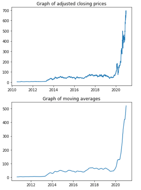program to plot the moving averages and adjust the closing price

# importing the matplotlib package 
import matplotlib.pyplot as plt

plt.subplots(0,0)
# Plotting the adjusted closing prices
plt.plot(adj_close)
plt.title("Graph of adjusted closing prices")

plt.subplots(0,1)
# Plotting the moving averages
plt.plot(m_av)
plt.title("Graph of moving averages")

Output:

Plotting Them Together

Code

# Python program to plot the moving averages and adjust the closing price

# importing the matplotlib package 
import matplotlib.pyplot as plt

# Plotting the adjusted closing prices
plt.plot(adj_close)

# Plotting the moving averages
plt.plot(m_av)

Output: