| |

K-means 1D clustering in PythonIn this article, K-means clustering in 1D?will be the main topic. To introduce the technique and illustrate the idea, a basic implementation in 1D?will be used. The notion will be expanded to N dimensions in the following post. This article will concentrate not just on the technique under discussion but also on the underlying code - in this case, Python. That is, this post is about K-means 1D clustering as much as it is about Python, or maybe even programming in general. In order to accomplish this, we will go line by line through the associated code to comprehend not just what it is doing but also how and why.
Although one-dimensional data isn't typically used for K-means clustering, it makes for a very straightforward example that shows how the process functions. The purpose of this post is to demonstrate how to use Python to display K-means clustering in 1 dimension, as indicated by the title. The Programme :This particular script aims for clarity above brevity, so some knowledge with Python or at least programming is anticipated, although the most of the information will be detailed in depth below. Both Python 2.x and Python 3.x should be compatible with the script, which also needs the numpy and matplotlib packages to be installed. Okay, let's get going. Create a file called kmeans1D_demo.py in your preferred IDE or text editor and then start by following the instructions. The no. of clusters we'll actually create, each containing pntsPerCluster points, is nmbrClusters. The (min, max) values provided by xCntrBounds will be used to position the centres of these clusters ("x" is our one dimension in our one-dimensional example). The "K" in "K-means" stands for the no.?of centroids, or clusters, that we want the algorithm to search for. Keep in mind that the algorithm looks for a different no. of clusters than we actually produce. This is actually a crucial point; in this instance, we actively create data clusters before allowing our K-means algorithm have a crack at it. However, we won't typically be producing the data in the real world. It will be up to us and/or our K-means algorithm to decide how many clusters the data needs to be divided into, i.e., what value of K to select, since we won't know precisely how many clusters exist, if any. The best value of K can be found using several techniques; however, we'll cover those in more detail later. In order to create an array of random floats in the range [0.0, 1.0], chosen from a continuous uniform distribution, it first uses the random sample function of the random module of Numpy (in contrast to a normal distribution). The next line converts these elements from the [0.0, 1.0] range to the xCntrBounds range. These variables serve as the centres of the point clusters that we'll create, which is accomplished in the following section of the code (every iteration of the loop here is generating a cluster of points and is storing them in different points). To do this, we use the numpy function randn(), which pulls from a normal distribution, and construct a standard deviation, stDev. The points will spread out as stDev's value increases, whereas a decrease in its value will result in clusters that are closer together. Play with this to observe how it affects the algorithm's capacity to distinguish across clusters. There are numerous strategies for determining the initial positions of our K centroids. This is significant since the result depends on the starting locations we choose. Any given set of data can be clustered in a variety of ways. The K-means method merely ensures that we will get a solution ("local optimum"), not necessarily the optimal answer (the "global optimum"). Nevertheless, as a general rule, selecting K distinct points at random from our data collection and using those as the initial centroid locations is a decent technique to establish the centroid locations. By selecting K distinct indices from the points array and saving the values at such indices in the centroids array, this is achieved. We will update centroids with the updated centroid locations after each algorithm iteration. Finally, using the function "assignPntsToCentroids()", we will assign each point in the collection to the cluster whose centroid it is closest to. In other words, we will iterate through points and, for each point, find which of the K centroids in centroids that point is closest to, and then hold the index pertaining to that centroid/cluster in the array classifications (since we are "classifying" the point as belonging to one of the K clusters).?A point in points is the equivalent of each categorization element. This means that if classifications[3] = 0, the fourth point, or points[3], is nearest to centroid 0, for whom the location is indicated by centroids[0]. The built-in absolute value method?abs()?can be used to calculate the path?between a given point and a particular centroid because this example only involves one dimension. Once we've defined our method assignPntsToCentroids(), we call it once to cluster the points according to the initial centroid coordinates that are already in centroids. The other key component of the process is to recalculate the centroid location for each cluster, and this section of program defines a function called reCalcCentroids() that does so. If sum(classifications == k) > 0, we first determine whether any points have actually been awarded to each cluster. If the sum of the components is at least 1, then at least one point is allocated to that cluster. The comparative statement classifiers == k returns an array with 1s at the indices where the?classifications represents k and 0s where it doesn't. The next sentence divides by the total no.?of points in the cluster to calculate the centroid. Division by zero is avoided by ensuring that the cluster contains at least one point. Since the purpose of this lesson is to display the algorithm, each cluster should be represented by a different colour. Utilizing the HSV colour space, which organises colours according to hue, saturation, and brightness value, is a clever approach to accomplish this for any arbitrary no. of clusters. A cone/cylinder can be used to symbolise these properties. As we round the cylinder, the colour changes. Red is represented by 0°, green by 120°, blue by 240°, and returning to red at 360°. A float from 0 to 1 represents the range 0°-360° in Python colorsys module. Then, using all but the final number, we split the hue spectrum [0, 1] into K+1 equally distanced values to get K different colours. This is due to the fact that the first and last numbers will both be 0, which in the HSV colour space represents the colour red. Then, we use the pyplot function subplots() to generate a figure with an axis. This function will return handles to the figure and axis objects, allowing us to subsequently obtain or alter the properties of the figure and axis. We would like to plot every cluster and its centroid in a separate colour in order to visualise the process. Additionally, we should be able to update every cluster following an algorithm iteration. To accomplish this, we'll use a for-loop to execute the plot() function of our axis for each cluster and centroid. This will initialise an empty matplotlib line object for each cluster and centroid. In essence, we use plot() to add a "line object" to the axis axe for every K clusters. The arguments we supply to plot() determine the characteristics of our line object. The x and y coordinates of the points we want to depict are the first two arguments to the plot() function. With ax.plot([], [],...), we initialise a line without any x or y data by supplying it empty arrays. The linestyle is determined by the keyword parameter ls; matplotlib is informed that we wish to plot the points without even a connecting line by ls='None'. The marker style is determined by the keyword argument marker. Any matplotlib colour specification can be used as the keyword argument colour. Here, we're using the colorsys method hsv_to_rgb to create an RGB tuple from our HSV colours(Note that colorsys was used to demonstrate that Python already has a built-in package to handle this capability; matplotlib also includes a colours module, matplotlib.colors, which could also convert HSV to RGB). In order to later change any of the aforementioned properties, plot() outputs a handle to the line object it just constructed. Of course, whenever we wish to update our plot, we must be able to access this line object handles afterwards. In order to accomplish this, we add the cluster and centroid line object handles to the corresponding lists, clusterPntsList and centroidPntsList. This keeps track of the items from our for-loop even after the loop has ended. The plot's lower left corner is then annotated with a blank line of text. This text will be used to show how many iterations the algorithm has gone through, and we'll update it using its handle, which I've named iterText. Just a simple function, is required to update the plot throughout each iteration of the algorithm. The value of the iterText annotation is set by our updatePlot() function using one input, the current iteration. The function first determines which points are a part of each cluster k, using that information to set the x data of the line object belonging to that cluster (which it obtains from clusterPntsList). An array of x coordinates and other?array of y coordinates are the two inputs that the set data() function requires. The y values are irrelevant because this is a 1D?example, so we set them all to 0. Note that since we had specified the line object colours and marker styles when we generated the line objects, we don't need to bother about doing so now. We only supply a single x value and a single y value to the set data() method of the centroid line object since every?cluster only has one centroid value. The plot is then saved as an image using the savefig() method. This will happen on each iteration of?while loop that we'll use to animate the algorithm. The animation will then be turned into a video using the photos. If you don't want to save photographs of the animation, you can comment out this line. NOTE : USING A WHILE LOOP FOR USING ANIMATION IN MATPLOTLIB OR TO ANIMATE VIDEOS IS NOT RECOMMENDED.When using a while loop to animate objects in Matplotlib is possible, it is not recommended. This is better accomplished with the animation module in matplotlib. Additionally pointless, the matplotlib.animation module already performs the task of manually producing a video and saving individual frames. In addition, we would like to show you how it's done the "hard way" before showing you how it's done correctly. Returning to the present code; In order to guarantee that all of our data points will be shown, we next specify the axis bounds of our plot. The updatePlot() function, which was previously defined, is then used to initialise the plot. Afterward, we activate Plt.ion() method's interactive charting. Ironically, by allowing the remainder of the code to continue running while the plot is open, this enables us to continuously update the plot without user intervention. Finally, to actually display the plot, a call to plt.show() is required. Finally, we put the algorithm into action. When the centroid positions stop shifting, the end condition has been satisfied. To ensure the while loop runs at least once, we construct the array last_Centroids and initialise it with a random set of values that differ from centroids. In other words, if we were using last_Centroids = centroids, last_Centroids and centroids will indeed point to the same object, modifying one would modify the other, and since they both point to the same object, they will always be equal, meaning the loop would only execute once. Take note that we use np.copy() instead of last_Centroids = centroids because that would point to it rather than create a copy of it. It's crucial to be aware of this peculiarity of numpy arrays. Now we can check the results after running the script. Try executing it more than once to observe the effects of various centroid initializations on the outcomes. Play with the settings by experimenting with different K values, cluster densities, and cluster standard deviations. The Complete Code:Output : 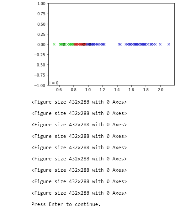
|
 For Videos Join Our Youtube Channel: Join Now
Feedback
- Send your Feedback to [email protected]
Help Others, Please Share


