| |

Gradient Descent Optimizer in PythonGradient Descent uses an iterative algorithm to find the optimal parameters of a model. Its main aim is to minimize the given function by finding the values of the parameters of that function. These are called optimal parameters. We can use gradient descent for a function of any dimension, such as 1-D, 2-D, or 3-D. In this tutorial, we will concentrate on determining the ideal parameters of the well-known equation, i.e., the linear regression equation, using the gradient descent algorithm.
We are now aware of the parameters we need for the algorithm. To fully grasp the working of gradient descent, let's map those parameters with the algorithm and manually work on an example. Let's take an example of the parabolic equation y = 4x2. This parabolic function is lowest when x = 0, or at x = 0, y = 0, as can be seen by putting these values in the function. As a result, the local minimum of our parabolic function y = 4x2 is at x = 0. Let's now look at the algorithm of the gradient descent optimizer and how we can use it to find the local minima of our parabolic function. Algorithm for Gradient DescentThe algorithm works in the direction based on the proportion of the function gradient's negative value at the present location (advance in the opposite direction of the gradient) to locate the local minima of any function. Gradient Ascent is the technique for reaching the function's local maximum value by traveling in steps proportional to the function gradient's positive value (moving in the direction of the gradient). Repeat this block until it converges to the required value. 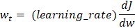
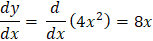
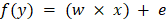
Step 1: We have to initialize all the important parameters first. Then we must derive the gradient function for our parabolic function y = 4x2. This is a basic derivation. 2x is the derivative of 4x2, so the derivative will be dy/dx = 8x. x0 = 4 (random value of x) learning_rate = 0.02 (This will determine the step size taken by the algorithm to reach the local minima) gradient = Step 2: For example, we will perform three iterations of the gradient descent function. For each iteration, we have to update the value of x based on the value of gradient descent in the previous iteration. Iteration 1: x1 = x0 - (learning_rate * gradient_equation) x1 = 4 - (0.02 * (8 * 4)) x1 = 4 - 0.64 x1 = 3.36 Iteration 2: x2 = x1 - (learning_rate * gradient_equation) x2 = 3.36 - (0.02 * (8 * 3.36)) x2 = 3.36 - 0.54 x2 = 2.82 Iteration 3: x3 = x2 - (learning_rate * gradient) x3 = 2.82 - (0.02 * (8 * 2.82)) x3 = 2.82 - 0.45 x3 = 2.37 We can see from the three gradient descent iterations that x is falling at each step and that by continuing the gradient descent algorithm for further iterations, it will gradually converge to 0, which is the required value. The next question is how many iterations an algorithm needs to converge to the local minima of the given function? There is an option for us to set the threshold value. This is the difference between the two values of x, the current and the previous one. The function will stop the iterations when this difference is less than the threshold value. We apply gradient descent to the cost functions of the machine learning and deep learning models. It aims to minimize that cost function. Now we know what goes on behind the scenes in working gradient descent. Let us now see its implementation in Python. As told earlier, we will minimize the linear regression model's cost function and find the best-fit line. In this case, our parameters will be w and b Prediction FunctionThe cost function in linear regression algorithms is the equation of a line, i.e., the equation So, the prediction function will be Here, x is used for independent feature y is used for dependent feature w is used for the weight associated with the independent feature e is used for error Cost FunctionMost machine learning models make some sort of prediction or classification. In both cases, the model gives some values as output. We check these predicted values against the observed values that we have with us. Loss in a model is defined as the difference between these two values, I.e., the predicted and the observed values. For linear regression, we calculate loss using the mean squared error formula. Mean squared error is calculated by finding the mean of the squared differences between the observed and the predicted values. The equation of the cost function is given below. 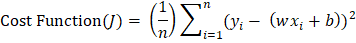
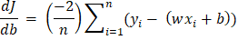
Here, n is the number of samples. Y is the predicted value, and y is the observed value. Partial Derivatives (Gradients) Now we will calculate the partial derivatives of the cost function with respect to the weight and the error terms. The result is: 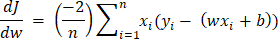
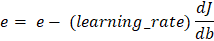
Parameter Updates The parameters will be updated using the formula that we used earlier. Subtract the result by multiplying the learning rate and its gradient from the parameter. 

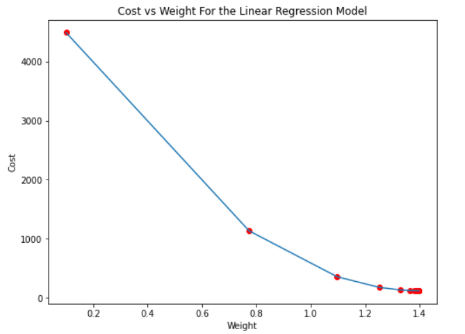
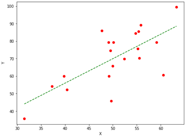
Implementing Gradient Descent in PythonFor the implementation of the above algorithm, we will define two functions. One will return the cost value using the cost function described above. This function will take the observed and predicted values of the dependent variable as parameters. The second function will be the one to implement the gradient descent algorithm. This function will take the independent and dependent variables as input parameters and return the optimal values of the weight and error parameters of the linear regression equation. Hence, it will give us the best-fit line for our data. We can tune the parameters' number of iterations, learning rate, and the stopping threshold values of the gradient descent function to make it more efficient. To implement these functions, we will create our data. We have taken random values which are almost linearly dependent. Using the gradient descent function, we will find the optimal parameters for the linear regression model equation to find the best-fit line for this data. The number of iterations specifies the number of times the function will update the values of weight and error; the stopping threshold is the threshold or the minimum value of the change in the cost or loss value for any two consequent iterations. Code Output: At iteration 1: The value of cost: 4490.368112564136, weight: 0.7732901495653765, and the error is: 0.023058581526390003 At iteration 2: The value of cost: 1131.6506097576817, weight: 1.0973277566276178, and the error is: 0.02933947690034616 At iteration 3: The value of cost: 353.6864536509919, weight: 1.2532789421408856, and the error is: 0.0323584432495475 At iteration 4: The value of cost: 173.49022435062597, weight: 1.3283343812503887, and the error is: 0.033807525620796475 At iteration 5: The value of cost: 131.75220717474858, weight: 1.3644567422091003, and the error is: 0.03450106252964878 At iteration 6: The value of cost: 122.08462343134752, weight: 1.3818415966647506, and the error is: 0.03483097452170135 At iteration 7: The value of cost: 119.84536542439749, weight: 1.3902085628198768, and the error is: 0.034985883049982396 At iteration 8: The value of cost: 119.32669605130852, weight: 1.394235447257572, and the error is: 0.03505656685253503 At iteration 9: The value of cost: 119.20655864249093, weight: 1.3961735600573946, and the error is: 0.03508671544159867 At iteration 10: The value of cost: 119.17873134396095, weight: 1.3971063998600626, and the error is: 0.03509735547518664 At iteration 11: The value of cost: 119.17228540809819, weight: 1.397555427176545, and the error is: 0.03509860655236391 At iteration 12: The value of cost: 119.170791938096, weight: 1.3977716077711553, and the error is: 0.0350953389803933 At iteration 13: The value of cost: 119.17044558479306, weight: 1.3978757251232417, and the error is: 0.03508989671506608 At iteration 14: The value of cost: 119.17036493281425, weight: 1.397925909268681, and the error is: 0.035083407843062374 At iteration 15: The value of cost: 119.17034582400478, weight: 1.3979501367245375, and the error is: 0.035076415283989484 At iteration 16: The value of cost: 119.1703409701581, weight: 1.3979618718813835, and the error is: 0.035069180331332335 At iteration 17: The value of cost: 119.17033941812645, weight: 1.3979675948100971, and the error is: 0.0350618287390411 |
 (Calculation of the gradient function)
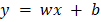
 For Videos Join Our Youtube Channel: Join Now
Feedback
- Send your Feedback to [email protected]
Help Others, Please Share


