Sklearn Regression Models

Machine learning is utilized to tackle the regression question using two different algorithms to perform regression analysis: logistic regression and linear regression. These are the most widely used regression approaches. Regression analysis approaches in machine learning come in many algorithms, and their use depends on the type of data and the analysis aim.

This tutorial will describe the various machine learning regression models and the circumstances in which we can apply each. This tutorial will undoubtedly aid us in grasping the regression modelling concept if one is a novice to machine learning.

Regression Models

In the supervised machine learning paradigm, the system is taught the results. The model's input and output variables are known to us, and both are used for training the algorithm. The algorithm is fed the true values in the training phase, and the machine learning model is trained to lower the prediction error. The two main supervised learning algorithm categories are regression (for the continuous target variable) and classification (for the discrete target variable).

A predictive modelling method called regression analysis examines the relationship between the target or dependent feature and the independent feature of a dataset. Various regression models are used depending on if the dependent and independent features exhibit a linear or a non-linear association between one another or if the target feature has continuous values. Regression analysis is frequently used to identify cause and effect relationships, forecast trends, time series forecasting analysis, and predictor strength.

Regression gives the result as continuous data. With the help of this technique, which is centered on characteristics, we may predict the patterns of the training data. The output is a real numerical number; however, it doesn't fall into any class or category. For instance, estimating property values depends on details like a home's size, locality, and development ratio, among many other things.

Types of Regression Analysis Techniques

Regression analysis approaches come in a wide variety, and factors, as discussed above, will determine which technique is used. Examples of these factors are the regression line pattern and the number of independent features.

The many regression approaches are listed below:

Linear Regression
Logistic Regression
Ridge Regression
Lasso Regression
Polynomial Regression
Bayesian Linear Regression
Decision Tree Regression
Support Vector Regression
Gradient Boosting Regression

Linear Regression

A machine learning method called linear regression establishes a linear relationship among one or multiple independent features and a particular dependent feature to forecast the dependent feature's best value by predicting the linear equation's variables' coefficients.

The simple linear regression model calculates the best fitting line for a dependent feature (y) and a single independent feature (x). The accompanying straight-line equation defines it.

m is the regression coefficient. It indicates how much we anticipate y to alter as the value of x changes. The regression model determines the optimal intercept (c) value and regression coefficients to minimize the error (e).

The algorithm finds the optimum values of the parameters by reducing the error between the actual values of target variable y and the values predicted by the model. The ordinary least squares approach is used to calculate the error. It can accommodate many input variables present in the dataset.

Code

# Python program how to perform a linear regression (Simple Regression and Multiple Regression)

# Importing the required libraries
import numpy as np
import pandas as pd
from sklearn import preprocessing
from sklearn.model_selection import train_test_split
from sklearn.datasets import load_diabetes
from sklearn.linear_model import LinearRegression


# Loading the diabetes dataset
diabetes = load_diabetes()

# Checking the target feature is a continuous data
print(diabetes.target[:10])

# Creating a dataframe
dataset = pd.DataFrame(data = diabetes.data, columns = diabetes.feature_names)

# Adding the target variable to the dataset
dataset["target"] = diabetes.target

# Separating the dependent and independent features
X = dataset.iloc[:, :-1].values
Y = dataset.iloc[:, -1].values


# Separating the data for training and testing the model
X_train, X_test, Y_train, Y_test = train_test_split(X, Y, test_size = 0.3, random_state = 15)

# Creating an object of the Linear Regression model class
l_reg = LinearRegression()

# Fitting the training data to the linear regression model
# Creating a Simple Linear Regression model using only one independent feature of the training dataset
l_reg.fit(X_train[:, 2:3], Y_train)

# Printing the R-square for the simple linear regression model by passing the unseen or the testing data
score = l_reg.score( X_test[:, 2:3], Y_test )
print("The r-square score of the Simple Linear Regression model: ", score)

# Creating a Multiple Linear Regression model using all the independent features
l_reg.fit(X_train, Y_train)

# Finding the predicted values
Y_pred = l_reg.predict(X_test)

# Creating a dataframe for the coefficient values of the independent features
coef = pd.DataFrame(data = dataset.iloc[:,:-1].columns, columns = ["Features"])
coef["Coefficients"] = l_reg.coef_
coef.loc[0] = ["Intercept", l_reg.intercept_]
coef

Output:

[151.  75. 141. 206. 135.  97. 138.  63. 110. 310.]
The r-square score of the Simple Linear Regression model:  0.3195508704110651

	Features	Coefficients
0	Intercept	150.559849
1	sex	-207.159699
2	bmi	545.523615
3	bp	282.960253
4	s1	-1195.950976
5	s2	580.404692
6	s3	404.413845
7	s4	431.717208
8	s5	871.098497
9	s6	118.346669

Logistic Regression

Logistic Regression is another type of regression modelling technique employed if the dependent feature is discrete, such as true or false, 0 or 1, etc. As a result, the dependent variable has only two possible values to take, and a sigmoid curve depicts the association between the target and input variables.

The logistic regression algorithm uses the logit function to quantify the relationship between the target and input variables.

Code

# Python program to create a regression model using Logistic Regression algorithm

# Importing the required modules
from sklearn.datasets import load_iris
from sklearn.metrics import accuracy_score
from sklearn.model_selection import train_test_split
from sklearn.linear_model import LogisticRegression

# Loading the iris dataset
X, Y = load_iris(return_X_y = True)

# Separating the data for training and testing the model
X_train, X_test, Y_train, Y_test = train_test_split(X, Y, test_size = 0.4, random_state = 15)

# Creating an object of the Logistic Regression model class
log_reg = LogisticRegression(random_state = 10)

# Fitting the training data to the logistic regression model
log_reg.fit(X_train, Y_train)

# Predicting the values for the unseen data
Y_pred = log_reg.predict(X_test)

# Computing the accuracy score of the Logistic Regression model
scores = accuracy_score(Y_test, Y_pred)
print(scores)

Output:

1.0

Ridge Regression

When independent features have a high correlation value, the Ridge regression algorithm predicts the target variable. This is because, for non-collinear variables, the least square estimates an unbiased answer. However, there may be a bias component if the collinearity is strong. As a result, a bias grid is induced in the equation of Ridge Regression. This powerful regression method makes the constructed model much less likely to overfit.

Code

# Python program to create regression model using Ridge Regression algorithm

# Importing the required modules
from sklearn.datasets import load_diabetes
from sklearn.metrics import r2_score
from sklearn.model_selection import train_test_split
from sklearn.linear_model import Ridge

# Loading the iris dataset
X, Y = load_diabetes(return_X_y = True)

# Separating the data for training and testing the model
X_train, X_test, Y_train, Y_test = train_test_split(X, Y, test_size = 0.4, random_state = 15)

# Creating a Logistic Regression model class object. The model will be using solver = 'svd.'
r_reg = Ridge(solver = 'svd', random_state = 10)

# Creating another model with solver = 'lsqr.'
# This is the fastest solver based on the least square routine of sklearn
r_reg1 = Ridge(solver = 'lsqr', random_state = 10)

# Fitting the training data to the Ridge regression model
r_reg.fit(X_train, Y_train)
r_reg1.fit(X_train, Y_train)

# Predicting the values for the unseen data
Y_pred = r_reg.predict(X_test)
Y_pred1 = r_reg1.predict(X_test)

# Computing the accuracy score for both the models
print('Accuracy score for solver = "auto": ', r2_score(Y_test, r_reg.predict(X_test).round(5)))
print('Accuracy score for solver = "lsqr": ', r2_score(Y_test, r_reg1.predict(X_test).round(5)))

Output:

Accuracy score for solver = "auto": 0.40731258229249656
Accuracy score for solver = "lsqr": 0.4073540170017558

Lasso Regression

One regression model applied in learning algorithms that integrate feature selection, and normalization procedures are called Lasso Regression. The absolute value of the regression coefficient is not considered. As an outcome, unlike in Ridge Regression, the independent features' coefficient value is close to zero.

Lasso Regression involves feature selection. This process permits selecting a group of variables from the given dataset, which will cause more change in the model than other variables. In Lasso Regression, all other features are set to zero except for the features required to make good predictions. This step helps keep the model from overfitting. When the collinearity value of the dataset's independent factors is severe, lasso regression only chooses one variable and reduces the coefficients of the other variables to zero.

Code

# Python program to create regression model using the Lasso Regression algorithm

# Importing the required modules
from sklearn.datasets import load_diabetes
from sklearn.metrics import r2_score
from sklearn.model_selection import train_test_split
from sklearn.linear_model import Lasso

# Loading the iris dataset
X, Y = load_diabetes(return_X_y = True)

# Segregating the training and testing data
X_train, X_test, Y_train, Y_test = train_test_split(X, Y, test_size = 0.3, random_state = 9)

# Creating an object of the Lasso Regression model class
l_reg = Lasso(random_state = 9)

# Fitting the training data to the Lasso regression model
l_reg.fit(X_train, Y_train)

# Predicting the values for the unseen data
Y_pred = l_reg.predict(X_test)

# Computing the accuracy score for both the models
print('The accuracy score of the model is: ', r2_score(Y_test, l_reg.predict(X_test).round(5)))

Output:

The accuracy score of the model is: 0.40131502999775714

Polynomial Regression

Another regression analysis method used in learning algorithms is polynomial regression. This method is similar to multiple linear regression with some minor adjustments. The n^th degree in the polynomial regression defines the link between the independent and dependent features, X and Y.

As a predictor, it uses a linear model for regression; we scale the features using a polynomial scaler function of sklearn. The algorithm of polynomial regression, like linear regression, uses the Ordinary Least Squares method to compare the errors of the lines. Instead of being a straight line in polynomial regression, the best-fitting line has a curve and depending on the power of X or the value of n, it crosses the data points.

While trying to achieve the lowest value of the OLS equation and find the best-fitting curve, the polynomial regression model is prone to overfitting. Evaluating the different regression curves, in the end, is advised because extrapolating higher polynomials can produce odd results.

The dataset is available here- https://github.com/content-anu/dataset-polynomial-regression

Code

# Python 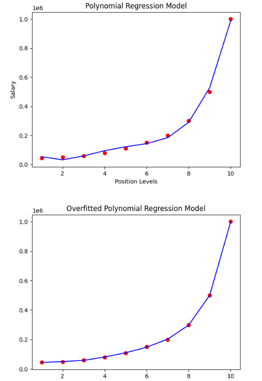program to perform the Polynomial Regression using sklearn

#importing the required libraries
import numpy as np
import pandas as pd
from sklearn.preprocessing import PolynomialFeatures
from sklearn.linear_model import LinearRegression
import matplotlib.pyplot as plt
%matplotlib inline

#importing the uploaded CSV dataset
data = pd.read_csv('Position_Salaries.csv')

# Seperating the independent and dependent features of the dataset
X = data.iloc[:,1:2].values
Y = data.iloc[:,2].values

# Creating an instance of the Polynomial Scaler
poly_reg = PolynomialFeatures(degree = 4)

# Fitting and transforming the X dataset to the Polynomial Scaler
X_polynomial = poly_reg.fit_transform(X)

# Creating a Linear regression model instance
lreg = LinearRegression()
lreg.fit(X_polynomial, Y)

#Visualisng the Polynomial regression model
plt.scatter(X, Y, color = 'red')
plt.plot(X, lreg.predict(poly_reg.fit_transform(X)), color = 'blue')
plt.title('Polynomial Regression Model')
plt.xlabel('Position Levels')
plt.ylabel('Salary')
plt.show()

# Using a higher degree polynomial to show overfitting
poly_reg1 = PolynomialFeatures(degree = 7)
X_polynomial1 = poly_reg1.fit_transform(X)
lreg1 = LinearRegression()
lreg1.fit(X_polynomial1, Y)
plt.scatter(X, Y, color = 'red')
plt.plot(X, lreg1.predict(X_polynomial1), color = 'blue')
plt.title('Overfitted Polynomial Regression Model')
plt.show()

Output:

Bayesian Linear Regression

One of the regression models used in machine learning, Bayesian Regression, calculates the magnitude of the regression coefficients using the Bayes theorem. Rather than locating the least squares, this regression approach determines the variables' posterior distribution. Like the linear regression and ridge regression methods, the Bayesian linear regression method is much more robust than simple linear regression.

Code

# Python program to perform Bayesian Regression

# Importing modules that are required
from sklearn.datasets import load_boston
from sklearn.model_selection import train_test_split
from sklearn.metrics import r2_score
from sklearn.linear_model import BayesianRidge
   
# Loading the Boston dataset
X, Y = load_boston(return_X_y = True)
   
# Splitting the training and testing datasets
X_train, X_test, Y_train, Y_test = train_test_split(X, Y, test_size = 0.3, random_state = 16)
   
# Creating an instance of the model and training it
br = BayesianRidge()
br.fit(X_train, Y_train)
   
# Predicting values for the unseen data, i.e., the testing data
Y_pred = br.predict(X_test)
   
# Computing the R-square score for the model
print(f"The r2 score of the model is: {r2_score(Y_test, Y_pred)}")

Output:

The r2 score of the model is: 0.6312926702997255

Elastic Net Regression

Elastic net regression is a regularised linear regression approach. It inserts the L1 and L2 costs to the loss function while training by linearly combining both. It blends lasso and ridge regression by giving each penalty the proper weight, enhancing predictive accuracy.

Alpha and Lambda are the two configurable hyperparameters for elastic nets. Lambda controls the proportion of the weighted total of the two penalties that determines the model's effectiveness. In contrast, the alpha parameter controls the weight assigned to each penalty individually.

Code

# Python program to perform Elastic Net Regression algorithm

# Importing the required libraries
from sklearn.linear_model import ElasticNet
import numpy as np

# Constructing an Elastic Net regression model having the hyperparameter value of alpha = 0.1
el = ElasticNet(alpha = 0.1)

# Preparing the input data
X = np.array([[2, 2], [2, 3], [2, 4], [3, 2], [3, 3], [3, 4]])

# Preparing the target variables
y = [ 7, 9, 11, 8, 10, 12]

# Fitting the data to the model
el.fit(X, y)

# Printing the coefficients of the model
print(el.coef_)

# Printing the intercept of the best fitting line
print(el.intercept_)

# Prediting value of a sample data
print(el.predict([[4, 4]]))
print(el.predict([[0, 0]]))

Output:

[0.66666667 1.79069767]
2.461240310077521
[12.29069767]
[2.46124031]

Decision Tree Regression

It is possible to represent judgments and all of their probable consequences, covering outcomes, input penalties, and utility, using a decision-making tool called a decision tree.

The supervised learning methods group includes the decision-tree strategy, and it functions with output results that are categorical and continuous values.

Decision Tree Regression: Decision tree regression develops a model to forecast future data to provide relevant continuous output by observing the attributes of an item and providing these attributes as input to the algorithm. Continuous output denotes the absence of a discrete outcome, i.e., output that is not only expressed by a discrete, well-known collection of figures or values.

Code

# Python program to show how to employ Decision Tree Regression

# Importing the required modules
import numpy as np
from sklearn.datasets import load_diabetes
from sklearn.tree import DecisionTreeRegressor
from sklearn.model_selection import train_test_split, cross_val_score

# Loading the diabetes dataset
X, Y = load_diabetes( return_X_y = True )

# Separating the whole dataset in the datasets to train and test the model
X_train, X_test, Y_train, Y_test = train_test_split(X, Y, test_size = 0.3, random_state = 10)

# Creating an object of the Decision Tree Regressor class
dtr = DecisionTreeRegressor(random_state = 10)
dtr.fit(X_train, Y_train)

# Computing the accuracy score of the Decision Tree model using the in-built cross_val_score method
scores = cross_val_score(dtr, X, Y, cv = 15)

# Printing the scores
print("Accuracy scores of the splits: ", scores)
print("The mean accuracy score of the model: ", np.mean(scores))

Output:

Accuracy scores of the splits: [-1.02298964 0.05276312 -0.74850198 -0.07277615 0.47050685 
0.3024374
 -1.31209035 -0.26358347 0.43173477 -0.19109809 -0.56778646 -0.61486148
 -0.11295867 
0.0408493 -0.26464188]
The mean accuracy score of the model: 
-0.25819978131125926

Support Vector Regression

Support Vector Regression (SVR) is unique compared to other regression models. It employs the Support Vector Machine (SVM, a classification approach) to forecast a continuous parameter. Support Vector Regression seeks to fit the best line inside a predetermined or threshold deviation value, as opposed to conventional linear regression models that aim to minimize the discrepancy between the estimated and actual value. In this respect, SVR categorizes all forecasting lines into two types: those that cross the error limit (a region divided by two parallel lines) and those that do not. When determining whether the discrepancy between the estimated value and the true value is beyond the error threshold, the lines that do not cross the error border are not considered (epsilon). The lines crossing the error threshold are added to the group of potential support vectors for forecasting an unknown value. We can better understand this idea if we look at the illustration below.

The kernel parameter of SVR is the most crucial It could be a Gaussian kernel, a Polynomial kernel, or a Linear kernel. We can choose a Polynomial or Gaussian kernel for our model as we have a non-linear property in the dataset, but in this case, we will select an RBF (Gaussian type) kernel.

Code

# Python 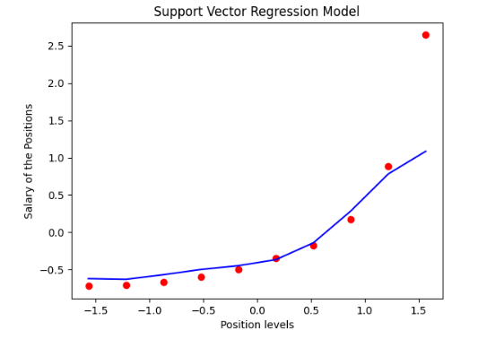program to apply Support Vector Regression

# Importing the required modules
import numpy as np
import matplotlib.pyplot as plt
import pandas as pd
from sklearn.preprocessing import StandardScaler
from sklearn.svm import SVR

# Importing the dataset
data = pd.read_csv('Position_Salaries.csv')

# Separating the target and independent variables
X = data.iloc[:,1:2].values.astype(float)
y = data.iloc[:,2:3].values.astype(float)

# Performing feature scaling
scaler = StandardScaler()
scaler1 = StandardScaler()
X = scaler.fit_transform(X)
y = scaler1.fit_transform(y)

# Creating an object of the Support Vector Regression class and fitting our dataset to construct the model
reg = SVR(kernel = 'rbf')
reg.fit(X, y)

# Predicting the value of a given initial condition
Y_pred = reg.predict([[7.5]])
print(Y_pred)

# Visualising the model using matplotlib plots
plt.scatter(X, y, color = 'red')
plt.plot(X, reg.predict(X), color = 'blue')
plt.title('Support Vector Regression Model')
plt.xlabel('Position levels')
plt.ylabel('Salary of the Positions')
plt.show()

Output:

Gradient Boosting Regression

We may apply a gradient boosting technique if there are difficulties with classification and regression methods. A predictive model is built using numerous smaller prediction models; these tiny models are often decision trees.

A loss function is necessary for the Gradient Boosting Regressor to perform. Gradient boosting regressors can handle a variety of predefined loss functions in addition to supporting customized loss functions; however, the loss function has to be differentiable.

Even though regression methods generally use the logarithmic function, squared errors can also be employed in regression techniques. We don't have to construct a loss function for each progressive boosting stage in gradient boosting algorithms; instead, we can choose whatever differentiable loss function.

Code

# Python program to perform regression using Gradient Boosting Regression algorithm

# Importing the required modules
import numpy as np
from sklearn.datasets import load_diabetes
from sklearn.ensemble import GradientBoostingRegressor
from sklearn.model_selection import cross_val_score

# Loading the diabetes dataset
X, Y = load_diabetes(return_X_y = True)

# Separating the training and validating datasets
X_train, X_test, Y_train, Y_test = train_test_split(X, Y, test_size = 0.3, random_state = 10)

# Creating an object of the Gradient Boosting Regressor class
gbr = GradientBoostingRegressor(n_estimators = 150, learning_rate = 1.0, max_depth = 2, random_state = 10)
gbr.fit(X_train, Y_train)

# Computing the accuracy score of the Gradient Boosting Regression model using the cross_val_score method
score = cross_val_score(gbr, X, Y, cv = 10)

# Printing the scores
print("Accuracy scores: ", scores)
print("The mean accuracy score is: ", np.mean(scores))

Output:

Accuracy scores: [-1.02298964 0.05276312 -0.74850198 -0.07277615 0.47050685 
0.3024374
 -1.31209035 -0.26358347 0.43173477 -0.19109809 -0.56778646 -0.61486148
 -0.11295867 
0.0408493 -0.26464188]
The mean accuracy score is: -0.25819978131125926

Regression Can Handle Linear Dependencies

A reliable method for forecasting numerical variables is regression. The machine learning techniques above include effective regression methods that can use the sklearn Python library to perform regression analysis and forecasting for various machine learning tasks.

But regression is a better option when a dataset has linear correlations between independent and dependent characteristics. Other regression algorithms, like neural networks, are employed to manage non-linear connections between data features because they can record non-linearity using activation functions.

Next TopicCOVID-19 Data Representation app using Tkinter in Python

← prev next →