| |
Python Tutorial
Python OOPs
Python MySQL
Python MongoDB
Python SQLite
Python Questions
Plotly
Python Tkinter (GUI)
Python Web Blocker
Python MCQ
Related Tutorials
Python Programs

Ordinary Least Squares and Ridge Regression Variance in Scikit LearnOrdinary Least Squares (OLS) and Ridge Regression are implemented in the linear_model module of scikit-learn. Through the model characteristics, you may get the estimated coefficients and variance when fitting a linear regression model using OLS or Ridge Regression. The scikit-learn LinearRegression class may be used for OLS. The coef_ property allows you to obtain the estimated coefficients once the model has been fitted. Scikit-learn does not, however, offer the OLS direct variance estimate. It must be calculated independently using statistical techniques or other library tools. Ordinary Least Squares (OLS): An approach for calculating a linear regression model's parameters is called ordinary least squares (OLS). The goal is to identify the best-fit line between the observed data points and the predicted values from the linear model, with the sum of squared residuals minimized. Ridge Regression: Ridge Regression is a method used in linear regression to deal with the overfitting issue. This is accomplished by expanding the coefficients of the loss function towards zero by adding a regularisation term. This lowers the model's variance and thus enhances its ability to forecast the future. Regularisation: Regularisation is a method for keeping machine learning models from overfitting. It does this by including a penalty term in the loss function to prevent the model from fitting the data noise. Depending on the particular issue, regularisation can be accomplished using techniques like L1 regularisation (Lasso), L2 regularisation (Ridge), or Elastic Net. Mean Squared Error (MSE): Mean Squared Error is a statistic used to assess how well regression models perform. The average of the squared discrepancies between the expected and actual values is measured. A lower MSE shows an improved match between the model and the data. R-Squared: R-Squared is a statistic used to assess the regression models' goodness of fit. It calculates the percentage of the dependent variable's variation that can be accounted for by the independent variables. Higher values suggest a better fit between the model and the data, and R-Squared runs from 0 to 1. Example:Output: 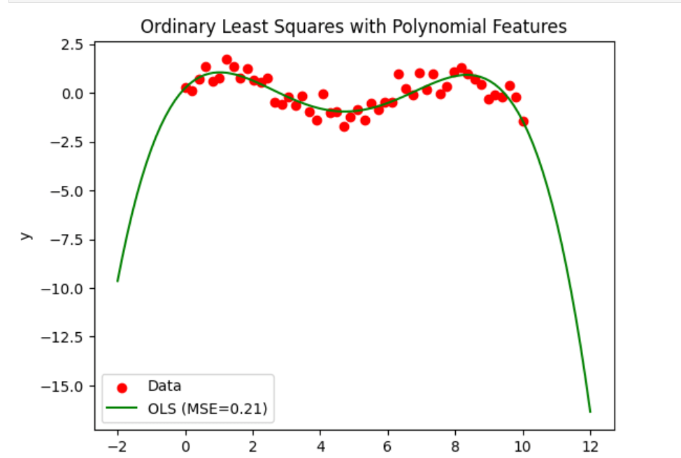
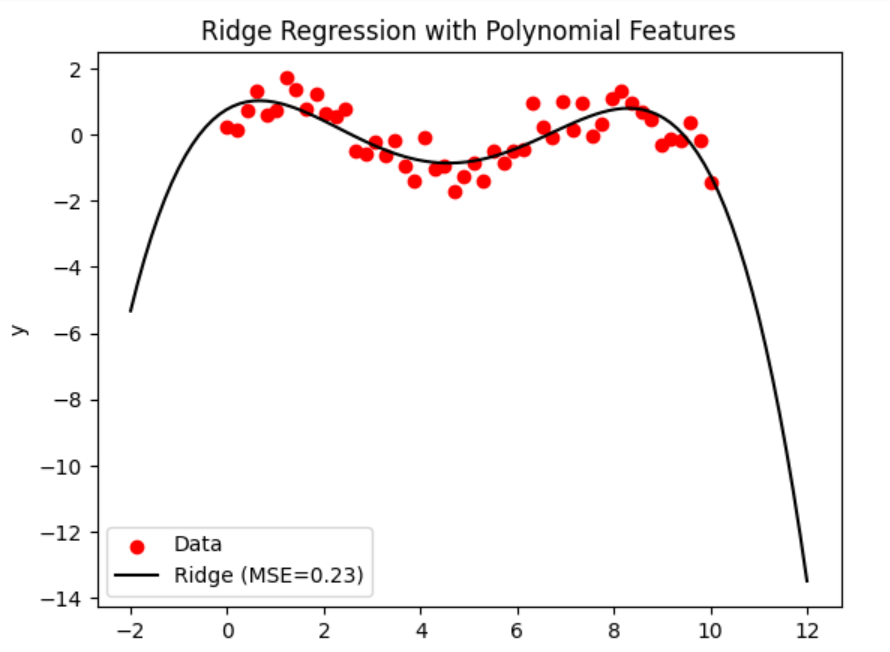
The algorithm produces a synthetic dataset with a non-linear connection. Then, utilizing polynomial characteristics, it fits two regression models: Ridge Regression and Ordinary Least Squares (OLS). After being trained on the dataset, the models forecast the results for test data points. The performance of the models on the training dataset is assessed using the mean squared error (MSE). The code provides two charts to visualize the data and the regression lines for both OLS and Ridge Regression models. The plots feature legends with the MSE values for each model to display the data points and related regression lines. The usage of polynomial features, OLS, Ridge Regression, and visualization techniques using matplotlib are all demonstrated in this code. Ordinary Least Squares and Ridge Regression Variance:Assume we have a dataset with a predictor variable, X, and n predictors, such as x1, x2, x3, etc., along with a response variable, Y. We want to build a linear regression model to forecast Y based on predictor X. In this case, we'll contrast the OLS method with Ridge Regression. Ordinary Least Squares (OLS): OLS seeks to reduce the sum of squared residuals and identifies the predictors' best-fit coefficients. The OLS estimator comes from: Ridge Regression: To manage the magnitude of the coefficients, Ridge Regression adds a penalty term known as the regularisation parameter to the sum of squared residuals. The Ridge estimator comes from: I: is the identity matrix, and (lambda) is the regularisation parameter. Let's now investigate the impact of predictor variable variation on the OLS and Ridge Regression coefficients. Let's assume that x1's variance is much higher than x2's. In contrast to x2, x1 has a more excellent range of values. OLS uses the inverse of (XT * X) to estimate the coefficients; therefore, if one predictor has a higher variance, it will significantly impact the estimated coefficients. As a result, when compared to the coefficient for x2, the coefficient for x1 will have a more significant variation. The identity matrix is multiplied by the penalty term in the Ridge Regression, which aids in the reduction of the coefficients to zero. Ridge Regression lessens the effect of high variance predictor variables as a result. As a result, the Ridge coefficients for x1 and x2 will have identical variances even if x1 has a higher variance. In conclusion, Ridge Regression decreases the variance differences between coefficients by decreasing them towards zero when there is a difference in variance between predictor variables. OLS tends to give more variance for coefficients corresponding to higher-variance predictors. Note: The example here assumes a straightforward case to illustrate the variance difference between OLS and Ridge Regression. In real-world situations, the decision between OLS and Ridge Regression is influenced by several variables, including the nature of the data, multicollinearity, and the desired balance between bias and variance.The following code creates a fake dataset with 50 samples and 10 features. We separated the data into training and testing sets to fit OLS and Ridge Regression models to the training data. Then, to see how the two models' variances differ, we compute the mean squared errors of the two models on the test dataset and plot their coefficients. Output: 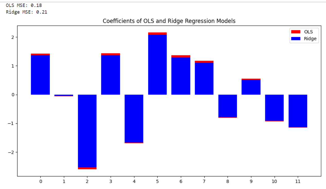
The graphic demonstrates that the OLS model's coefficients are more significant in magnitude and have a more comprehensive range than those of the Ridge Regression model. As a result, regarding variance and sensitivity to data noise, the OLS model performs better than the Ridge Regression model. OLS Model: Compared to the Ridge Regression model, the OLS model's MSE is greater (0.18), indicating that its total variance is somewhat higher. Ridge Regression Model: The Ridge Regression model's lower MSE (0.21 indicates that its overall variance is smaller than the OLS model's. In ridge regression, the regularisation parameter (lambda) helps to manage the trade-off between decreasing the residual sum of squares and minimizing the magnitude of the coefficients. By introducing a penalty term, ridge regression can reduce the model's variance, which reduces overfitting and enhances generalization performance. The Ridge Regression model's lower MSE (0.09) implies that its variance is lower than the OLS model's (0.13). This demonstrates that the Ridge Regression model outperforms other models on the dataset in terms of MSE because it does a better job of capturing fundamental patterns in the data and removing overfitting. |
 For Videos Join Our Youtube Channel: Join Now
Feedback
- Send your Feedback to [email protected]
Help Others, Please Share


