| |

Random Forest for Time Series ForecastingA well-liked and efficient ensemble machine learning approach is Random Forest. With organized (tabular) data sets, such as those in a spreadsheet or the relational database table, this algorithm is frequently used for predictive modelling through classification and regression. The time series data must first be converted into the form that can be used for training the supervised learning algorithms before using the Random Forest algorithm for performing the time series forecasting. Additionally, it necessitates employing a specialized evaluation method known as walk-forward validation since the k-fold cross-validation approach would yield hopefully biased findings. In this tutorial, you will learn how to use the Random Forest learning algorithm for time series forecasting. Random Forest EnsembleA collection of the decision tree models is called the random forest model. It is developed using the bootstrap aggregation called bagging on the decision trees and applies to classification and regression modeling. Multiple decision trees are constructed in the bagging process, and each tree is built from a separate bootstrapped sample of the primary training data. An instance may occur in more than one sample of the bootstrapped training datasets, known as a bootstrap sample. Bootstrapping is also described as "Sampling with replacement". As every decision tree is fitted on the little bootstrapped training datasets and, as a result, has a few varied outcomes, bagging is a successful ensemble method. The trees of the random forest ensemble are unpruned, in contrast to standard decision tree algorithms like the popular classification and regression trees model, also known as CART, which causes them to overfit the initial training dataset substantially. This is preferable since it makes every tree more distinctive and results in predictions with lower correlations or error rates. The model performs better when forecasts from all the ensemble decision trees are aggregated than when predictions from just one tree are considered. The average forecast across the ensemble's decision trees is an estimate on a regression line. A classification problem estimate is the class label that has received the most support from the ensemble of decision trees.
Like bagging, the random forest model entails building several decision trees using the bootstrap samples from the primary training dataset. In contrast to bagging, the random forest model also entails picking a selected group of input characteristics at every stage when the trees are divided. In order to choose a split point, every input attribute's value is often evaluated while building a decision tree. It pushes every decision tree into the ensemble to be more different by condensing the characteristics of a random data group that may be considered at every splitting point. The result is that every decision tree of the ensemble makes forecasts that are more dissimilar from one another or less correlated, which causes prediction mistakes. It frequently yields greater accuracy than bagged decision trees when the forecasts of these less correlated decision trees are aggregated to generate a forecast. Importing the required modulesTime Series Data PreparationWe can convert the time series data as supervised learning data. If given a timely ordered sequence of data, i.e., time series data, we can transform it into a supervised learning problem. This may be accomplished by utilizing the output attribute as the next data point of the data, and the input attributes, as the previous time steps. We may reconstruct the given time series data as a supervised machine learning problem by utilizing the data point at the most recent time step to forecast the data present at the following time step. We may reconstruct the given time series data as a supervised machine-learning problem. This format is known as a sliding window because it allows for creating fresh "samples" for supervised machine learning models by moving the window of the input variables and predicted outputs forward in time. Given the proper dimensions of the input and output time series data, we may automatically generate new frames for time series issues using the Pandas' shift() method. This would be a helpful tool since it would enable us to investigate various frames of the time series data using machine learning methods to determine which would provide models that perform better. With the supplied number of inputs and outputs instances, the function will take the time series represented as an array time series with one or multiple columns and turn it into a supervised machine learning problem. Code We will use this function later to convert the time series data to apply the Random Forest model. After creating the dataset, we need to be cautious while fitting and assessing a model using it. To fit the Random Forest model on the dataset from tomorrow and have it forecast past events, for instance, wouldn't be considered valid. The model has to be taught to forecast the future using historical data. As a result, techniques like kfold cross-validation that randomizes the given dataset while evaluating cannot be applied. We prefer to employ a method known as walk-forward cross-validation. The dataset is initially divided into the train and the test datasets by choosing a threshold point. For example, all the data, excluding the most recent 12 months, is utilized for training the model, and the most recent 12 months are utilized for testing that model in walk-forward cross-validation. By training our model on the training data and producing the first step prediction on the excluded test data, we may assess the model if we want to create a one-step prediction, such as one month. In order to update the model and have it forecast the second step data of the test dataset, we may then add the actual values from our test dataset to our training dataset. A one-step forecast for the whole test dataset may be obtained by repeating this procedure, through which an error measurement can be computed to judge the model's performance. The whole supervised learning dataset is required, together with the total number of rows to be used as the test dataset. It then steps through the test set, calling the random_forest_forecast() function to make a one-step forecast. An error measure is calculated, and the details are returned for analysis. Code We will define the train_test_split() function to split the training and testing datasets. The function is defined below. Code We will define the random_forest_forecast() function, which will use the sklearn library's Random Forest model, fit it to the provided training data, and return the predicted values for the given test dataset. Code We have created all the functions we need for the modeling and prediction. The next step is to load the dataset we will use to implement our methods. Random Forest for Time SeriesIn this final part, we will see how to implement the Random Forest regression to forecast the time series data values. We will use common univariate time series data to focus on the model's working. Also, we have prepared the methods for the univariate data only. To test the model, we will use a standard univariate time series dataset to make the predictions on the dataset. The code we have used can be used to understand the procedure of time series forecasting using the Random Forest model. We can extend the functionality to implement these methods on the multivariate data for multivariate forecasting, but we will need to make some changes to the methods. We will use the time series dataset of daily female births, which contains the number of females born in a month. The data is recorded for three years. One can download the dataset using the below link: Let us take a look at the dataset. These are the raw values. First, let us load this dataset in the current workspace and plot it. Below is the code to load and plot it. Code Output: 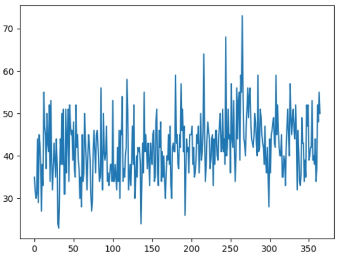
This is the line plot of the time series data. We cannot see any obvious trend or seasonality in the data. Now bringing everything together and running the model. Code Output: expected values = 42.0, predicted values = 45.583 expected values = 53.0, predicted values = 43.804 expected values = 39.0, predicted values = 41.545 expected values = 40.0, predicted values = 38.352 expected values = 38.0, predicted values = 42.782 expected values = 44.0, predicted values = 48.077 expected values = 34.0, predicted values = 42.743 expected values = 37.0, predicted values = 36.669 expected values = 52.0, predicted values = 37.75 expected values = 48.0, predicted values = 41.899 expected values = 55.0, predicted values = 43.849 expected values = 50.0, predicted values = 44.999 The MAE score is: 5.950666666666668 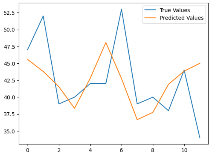
|
 For Videos Join Our Youtube Channel: Join Now
Feedback
- Send your Feedback to [email protected]
Help Others, Please Share


