| |

Python - Logistics Distribution in StatisticsProbability distributions are the cornerstone of statistical analysis, providing a structured way to describe and understand the variability within data. Among these distributions, the logistic distribution stands out as a versatile tool, particularly well-suited for modeling scenarios where outcomes are bounded between two limits. The logistic distribution finds applications in various fields, from predicting binary outcomes to understanding growth rates. In this post, we will investigate the features of the logistic distribution, decipher its complexities, and discover how to use Python to its fullest advantage. After this journey, you will have a firm understanding of how to use logistic distributions and apply them successfully to various statistical and predictive problems. What are Logistic Distributions?In statistics, a logistic distribution is a vital probability distribution used in modeling and analyzing various real-world phenomena. This distribution is particularly valuable when dealing with situations where outcomes are constrained within a specific range, often bounded between two values. The logistic distribution's distinctive S-shaped curve makes it an excellent choice for capturing sigmoid-like behavior, which is prevalent in numerous natural and social processes. Mathematically, the logistic distribution is defined by two key parameters: the location parameter μ (mu) and the scale parameter s (sigma). The location parameter represents the mean of the distribution, indicating where the peak of the curve is centered. The scale parameter determines the spread or variability of the distribution. A complex but elegant expression gives the probability density function (PDF) of the logistic distribution: 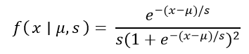
Here, x denotes the random variable, μ denotes the location parameter, and s denotes the scale parameter. Given the distribution's parameters, this function defines the likelihood of observing a particular value x. Moreover, the cumulative distribution function (CDF) of the logistic distribution is of paramount importance. It takes the form of the sigmoid function, which exhibits an S-shaped curve: 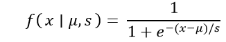
In this equation, F(x) represents the probability that the random variable x is less than or equal to a given value. The logistic distribution is a versatile tool for understanding and modeling bounded outcomes with sigmoidal tendencies, making it an indispensable asset in statistical analysis and predictive modeling. Applications of Logistics Distributions in StatisticsWith its unique properties and versatility, the logistic distribution finds many applications across various domains in statistics. This distribution's ability to model bounded outcomes and exhibit sigmoid-like behavior makes it an invaluable tool for addressing many real-world scenarios. Here are some notable applications of the logistic distribution in statistics: Logistic Regression: One of the logistic distribution's most well-known uses is in logistic regression. When attempting to forecast the likelihood of a binary result, this statistical strategy is used for binary classification problems. Logistic regression is built on the cumulative distribution function of the logistic distribution, sometimes called the logistic function or sigmoid function. It is perfect for modeling probabilities of binary outcomes since it converts the linear combination of predictor variables into a probability value between 0 and 1. Epidemiology and Medical Sciences: Logistic distributions are frequently used to model various medical phenomena, such as the probability of disease occurrence. For instance, logistic distributions can be employed to analyze the likelihood of a patient's medical condition based on risk factors and symptoms. These distributions can also be useful in epidemiology to model disease transmission probabilities and evaluate the effectiveness of interventions. Market Research and Economics: In market research, logistic distributions are applied to model consumer behaviors and preferences. For example, they can be used to analyze the likelihood of customers purchasing a product based on demographic or behavioral characteristics. In economics, logistic distributions find use in modeling outcomes with limited ranges, such as the probability of an individual defaulting on a loan or the likelihood of a stock price crossing a certain threshold. Ecology and Biology: Logistic distributions play a role in ecological modeling, particularly in population growth and carrying capacity scenarios. They can describe the growth of species populations up to a certain limit as resources become constrained. Logistic distributions might be used in genetics to model the probability of an organism inheriting a specific genetic trait. Psychology and Social Sciences: In psychology and social sciences, logistic distributions can help model behaviors that have natural limits. For instance, they can be applied to understand the likelihood of individuals adopting a certain behavior or responding to a particular stimulus. This can aid in predicting trends in human behavior and decision-making. Quality Control and Manufacturing: Logistic distributions can be utilized in quality control processes to model the probability of a manufactured product meeting certain specifications. This is particularly useful when the outcome is binary, such as pass/fail or acceptable/defective. Logistic distributions help assess the likelihood of a product falling within acceptable quality limits. In each of these applications, the logistic distribution's ability to capture the bounded and sigmoidal nature of various outcomes proves highly beneficial. By employing this distribution, statisticians and data analysts can gain insights, make predictions, and make informed decisions in various fields. Properties of Logistic Distribution
Python ImplementationImplement the logistic distribution in Python using the scipy.stats library, and then I'll explain the code step by step. First, make sure you have scipy installed; you can install it using pip if you haven't already: Below given a Basic Python implementation of the logistic distribution: Output: 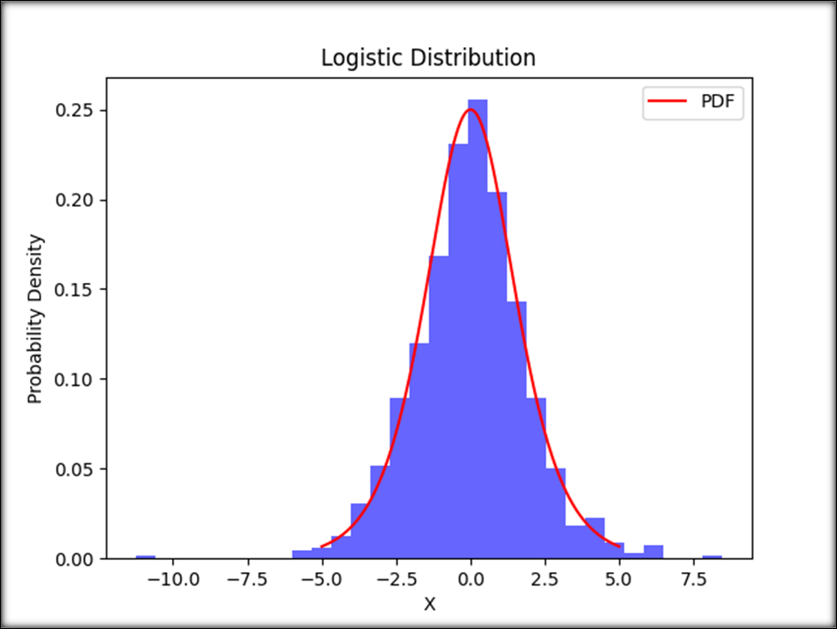
Explanation of the Code:
When you run this code, you'll get a visual representation of the logistic distribution and see how the generated data matches the theoretical distribution. This implementation can be a useful starting point for understanding and working with the logistic distribution in Python. ConclusionTo sum up, the logistic distribution is a potent and adaptable tool in the statistics toolbox. It is incredibly useful for simulating various actual processes due to its unique characteristics, including symmetry, sigmoidal shape, and the capacity to describe constrained outcomes. This distribution is a key building component in statistical analysis, used for anything from understanding growth rates to forecasting probabilities in logistic regression. With the help of the scipy.stats library's Python version, which we've looked at here, statisticians and data analysts may use the logistic distribution to obtain knowledge, forecast the future, and make defensible judgments in various fields. As you continue to explore the world of statistics and data science, the logistic distribution will remain a reliable tool for capturing and understanding the complex dynamics of many natural and social phenomena. The logistic distribution will continue to be a trustworthy instrument for capturing and comprehending the complex dynamics of many natural and social events as you further your statistics and data science studies. |
 . This demonstrates that the spread of the distribution is influenced by the scale parameter s. Larger values of s result in larger spreads.
 For Videos Join Our Youtube Channel: Join Now
Feedback
- Send your Feedback to [email protected]
Help Others, Please Share


