| |

Curve Fit in PythonIntroductionCurve fitting is a kind of optimization that finds an optimal parameter set for a defined function appropriate for a provided collection of observations. Different from supervised learning, curve fitting needs us to define the function mapping the examples of inputs to outputs. The function which use to map is also known as the basis function, and it can form anything of our preferences, such as a straight line (linear regression), a curved line (polynomial regression), and much more. This mapping function offers the flexibility and control in order to define the form of the curve, where the process of optimization is utilized in order to find the particular optimal arguments of the function. In the following tutorial, we will understand what curve fitting is and how we can perform it in Python. By the end of the tutorial, we will understand the following:
Understanding Curve FittingAs we discussed earlier, Curve fitting is a problem of optimization that allows us to find a line that is appropriate for a set of observations. It becomes easier when we think of a curve fitting in two dimensions as a graph. Suppose we have collected the data examples from the problem domain, including inputs and outputs. The x-axis of the graph acts as an independent variable that is the input to the function. On the other side, the y-axis of the graph acts as a dependent variable that is the output of the function. We may not know the function's form that maps examples of inputs to outputs; however, we can approximate the function using a standard form of function. Curve fitting includes the following stages:
Error is estimated using the observation provided by the domain and passing the inputs to the candidate objective function and estimating the output. The calculated output is compared to the experimental output. Once we have done fitting, we can utilize the basis function in order to interpolate or extrapolate the new points in the domain. It is general to execute a sequence of values of input using the basis function in order to estimate a sequence of outputs. After that, we make a line plot based on the result demonstrating the variance between the input and output and fitting the line on the observed points. The explanation for curve fitting is the form of the basis function. A straight line between inputs and outputs can be described using the formula given below: y = a × x + b Where y is the estimated output, x is the input, and a and b are the arguments of the basis function found with the help of an optimization algorithm. This equation is known as a Linear Equation as it is a weighted addition of the inputs. In a model of the linear regression, these arguments are indicated as coefficients, whereas in a neural network, these arguments are termed as weights. We can generalize this equation to any number of inputs, implying that the notion of curve fitting is not fixed to two dimensions (where one is input and the other is output). However, it could contain multiple variables for input. For instance, the formula for a line objective function for two input variables may appear as shown below: y = a1 × x1 + a2 × x2 + b It is not necessary that the equation appears to be a straight line. We can define curves to the objective function by inserting exponents. For instance, we can insert a squared version of the input weighted by another argument as described below: y = a × x + b × x2 + c This equation is termed polynomial regression, and the squared term refers to the second-degree polynomial. This type of linear equations can be fit by diminishing least squares and estimated analytically, which implies that we can find the argument's optimal values with the help of some linear algebra. Some of us might also want to include other mathematical functions in the equation, like sin, cos, tan, and many more. Each of the terms is weighted using an argument and added to the whole equation to produce the following output: y = a × sin(b × x) + c By adding the arbitrary mathematical functions to the objective function, we can't estimate the arguments analytically; however, we will require to utilize an algorithm for iterative optimization. This equation is considered as Non-Linear least squares because the mapping function is not convex anymore (it is Non-Linear) and not relatively easier to solve. Since we have successfully understood what curve fitting is, it is time for us to head onto understanding how curve fitting can be performed in Python. Performing Curve Fitting in PythonCurve Fitting can be performed for the dataset using Python. Python provides an open-source library known as the SciPy package. This SciPy package involves a function known as the curve_fit() function used to curve fit through Non-Linear Least Squares. The curve_fit() function takes the same input as well as output data as parameters in addition to the name of the objective function to utilize. The objective function must include examples of input data and few quantities of parameters. The parameters that are left remaining will become the coefficient or weight constants that a Non-linear Least Squares optimization process will optimize. Let us consider an example demonstration to understand this very concept. Suppose we have few observations from the domain loaded as x number of input variables and y number of output variables. Syntax: Now, we have to design an objective function in order to fit a line to the data and implement it as a function in Python that accepts inputs as well as the parameters. Let us assume that the function is a straight line, which would appear as shown below: Syntax: Once the function is defined, we can call the curve_fit() function in order to fit a straight line to the dataset with the help of the defined mapping function. The curve_fit() function will return the optimal values for the objective function. For example, the values of coefficient. The function will also return a co-variance matrix for the calculated arguments; however, this can be ignored for a moment. Syntax: Once the fitting is done successfully, we can utilize the optimal arguments and the objective function mapping() in order to evaluate the output for any subjective input. This function might involve the outputs for the examples we have already gathered from the domain. It might involve some newer values that can interpolate the observed values. It might also involve the extrapolated values outside the reach of the observed values. Syntax: Since we have understood how to utilize the API for curve fitting, let us look at a working example. Working Example for Curve Fitting in PythonLet us begin by importing the necessary packages and libraries for the project. Syntax: Once we are done importing the packages, we need test data for the program in order to implement the curve fitting. So, we are defining basic input data x and output data y as shown below. Syntax: After then, we will define some mapping functions in order to utilize the curve_fit() method and verify their differences in the fitting. We will utilize the equations shown below as the mapping functions:
The procedure for the same is described in the following syntax: Syntax: Fitting the data using the curve_fit() function is pretty simple that provides the mapping function, data x, and y, respectively. The curve_fit() method will return optimal arguments and calculated co-variance values as an output. Syntax: Output: Arguments: [-0.08139835 0.8636481 11.1362229 ] Co-Variance: [[ 2.38376125e-04 -3.81401800e-03 9.53504499e-03] [-3.81401800e-03 6.55534344e-02 -1.88793892e-01] [ 9.53504499e-03 -1.88793892e-01 7.79966692e-01]] As we can observe, the curve_fit() function evaluated the optimal arguments and the Co-Variance. We have then printed these values for the users. We will begin fitting the data by configuring the objective function and the data x and y into the curve_fit() method and get the resultant data containing the argument values for a, b, and c. Since we are not using the values of Co-Variance here, we can skip it. After that, we will estimate the y fitted by utilizing the derived a, b, and c values for each function. Syntax: At last, we will plot the graph in order to verify the differences visually. The syntax for same is shown below: Syntax: The Resultant Graph for the program is given below: Graph: 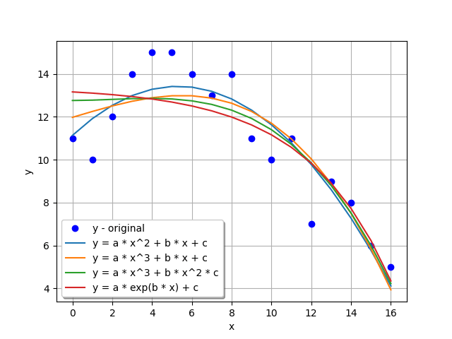
Next TopicConverting CSV to JSON in Python
|
 For Videos Join Our Youtube Channel: Join Now
Feedback
- Send your Feedback to [email protected]
Help Others, Please Share


