| |

Deep ConvNets Architectures for Computer VisionGood ConvNets are monstrous machines with many hidden layers and millions of parameters. 'Higher the number of hidden layers, the better the network' is really a terrible maxim. Among the well-known networks are ResNet, AlexNet, VGG, Inception, and others. Why are these networks so effective? How have they been created? They have the structures they have for what reason? One is curious. These questions don't have an easy solution, and one blog article can't possibly cover them all. However, I will attempt to address some of these queries in this article. It will take some time to understand how to create a network architecture and much more time to explore on your own. Let's first put things in context, though: Why do ConvNets outperform traditional Computer Vision?The process of placing a given image into one of the pre-established categories is known as image categorization. The feature extraction and classification modules make up the traditional pipeline for classifying images. The process of feature extraction entails taking the distinction between the many categories under consideration and extracting a higher degree of information from the raw pixel values. Unsupervised feature extraction is used in this case, meaning that the classes of the image have no bearing on the data gleaned from the pixels. GIST, HOG, SIFT, LBP, and other enduring and popular characteristics are a few examples. A classification module is trained using the photos and the labels that go with them once the feature has been retrieved. SVM, Logistic Regression, Random Forest, decision trees, etc. are a few examples of this module. This pipeline has the drawback that the feature extraction cannot be altered in accordance with the classes and pictures. Therefore, regardless of the type of classification approach used, the accuracy of the classification model suffers greatly if the chosen feature lacks the representation necessary to identify the categories. Picking various feature extractors and creatively combining them to achieve a superior feature has been a recurrent motif in the state-of-the-art after the typical pipeline. However, in order to adjust parameters in accordance with the domain and achieve a respectable degree of accuracy, this requires too many heuristics and manual labour. When I say decent, I mean having nearly human precision. Because of this, it has taken years to develop a good computer vision system (such as OCR, face verification, picture classifiers, object detectors, etc.) that can function with the vast range of data found in actual applications. For a corporation (a client of my start-up), we once delivered better results utilizing ConvNets in six weeks than it had taken them to do so using conventional computer vision. The fact that this approach is so different from how people learn to recognize objects is another issue with it. A newborn is unable to see his environment at birth, but as he develops and absorbs information, he learns to recognize objects. This is the underlying principle of deep learning, which lacks an internal feature extractor that is hard-coded. It integrates the modules for extraction and classification into a single integrated system, where it learns to separate representations from the pictures based on discrimination and categorize them using supervised data. Multilayer perceptrons, also known as neural networks, are one such system and consist of numerous layers of neurons that are tightly coupled to one another. Because there are so many parameters in a deep vanilla neural network, it is hard to train one without overfitting the model because there aren't enough training samples. Using a sizable dataset like ImageNet, however, Convolutional Neural Networks (ConvNets) allow for the task of training the whole network from the start. The sharing of parameters between neurons and sparse connections in convolutional layers are to blame for this. This illustration 2, for instance, shows it. In the convolution procedure, the 2-D feature map's parameters are shared, and the neurons in one layer are only locally linked to the input neurons. a. Accuracy: An intelligent machine must be as accurate as feasible if you want it to function properly. The fact that "accuracy not only depends on the network but also the amount of data available for training" is a reasonable question to pose in this context. In order to compare these networks, we use the ImageNet standard dataset. The continuing ImageNet project presently has 14,197,122 photos over 21841 distinct categories. Since 2010, the ImageNet dataset has hosted an annual visual recognition competition where contestants are given access to 1.2 million photos from 1,000 distinct classifications. Therefore, utilizing these 1.2 million photos from 1000 classes, each network architecture reports accuracy. b. Computation: The majority of ConvNets demand a lot of memory and processing power, especially while training. Consequently, this becomes a significant issue. Similar to this, if you want to deploy a model to operate locally on a mobile device, you must take into account the size of the final trained model. As you can expect, a network that uses more computing is able to deliver more accurate results. Therefore, precision and calculation are continuously in competition. In addition to these, there are several more variables, such as how simple it is to train a network and how effectively it generalizes. The networks listed below are the most well-known ones; they are shown in the sequence in which they were released, and they also improved in accuracy as they went along. AlexNetOne of the first deep networks to improve ImageNet Classification accuracy significantly above conventional approaches was this design. It has three completely linked layers after the first five convolutional layers. 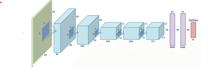
The non-linear component of AlexNet, developed by Alex Krizhevsky, employs Rectified Linear Units (ReLu) rather than Tanh or Sigmoid functions, which were previously the norm for conventional neural networks. ReLu is supplied by f(x) = max(0, x) The benefit of the ReLu over the sigmoid is that it trains significantly more quickly than the latter since the updates to the weights essentially cease to exist when the derivative of the sigmoid decreases in size in the saturation area. A vanishing gradient issue is what this is. ReLu layer is added to the network after every fully connected (FC) and convolutional layer. 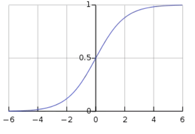
By adding a Dropout layer after each FC layer, this architecture also reduced over-fitting, which was an issue. Each neuron in the response map receives a separate application of the dropout layer, which has a probability (p) attached to it. With probability p, it deactivates the activation at random. 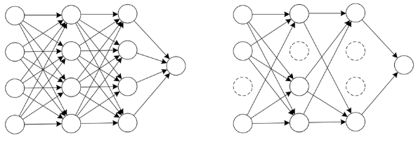

How does DropOutwork?The dropout and demonstrate outfits have a comparable reasonable structure. Various arrangements of neurons that are switched off because of the dropout layer address different plans, and these different models are prepared simultaneously with loads doled out to every subset and the total of the loads being one. The quantity of subset structures made for n neurons connected to DropOut is 2n. Basically, this implies that forecasts are arrived at the midpoint of different model gatherings. This offers an orderly strategy for model regularization, helping with forestalling over-fitting. One more method for taking a gander at DropOut's value is that since neurons are haphazardly chosen, they will quite often stay away from co-adjusting to each other, permitting them to gain critical qualities separated from each other. VGG16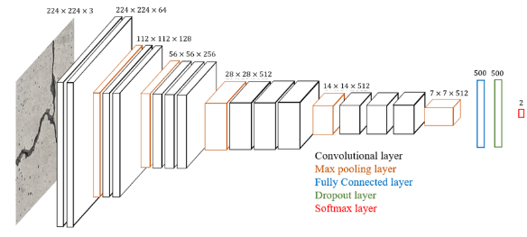
The VGG bunch at Oxford is the wellspring of this design. It beats AlexNet by successively subbing various 3X3 bit estimated channels for enormous 11 and 5-portion measured channels in the first and second convolutional layers, separately. Various non-direct layers increment the profundity of the organization, permitting it to learn more complicated highlights at a lower cost. This makes numerous stacked more modest size portions better compared to one with a bigger size part for a given responsive field (the viable region size of the information picture on which the result depends). You can see that blocks with a similar channel size applied ordinarily are remembered for VGG-D to remove more perplexing and delegate qualities. After VGG, blocks and modules spread all through the organizations. Three completely connected layers come after the VGG convolutional layers. After each sub-testing/pooling layer, the organization's broadness ascends by a component of 2, beginning at a low worth of 64. On ImageNet, it gets a main 5 exactness of 92.3%. GoogLeNet/Inception:Despite the fantastic accuracy that VGG achieves on the ImageNet dataset, its implementation on even the smallest GPUs is problematic because of the enormous computing demands, both in terms of memory and time. Due to the convolutional layers' wide breadth, it becomes ineffective. For instance, the computation order is 9X512X512 for a convolutional layer with a 3X3 kernel size that accepts 512 input channels and outputs 512 channels. Every output channel (512 in the example above) is connected to every input channel during a convolutional operation at a single place; for this reason, the architecture is referred to as having a dense connection. The GoogLeNet is based on the hypothesis that the majority of deep network activations are either redundant or unneeded (value of zero) due to correlations. As a result, the deep network's most effective design will feature sparse connections between activations, meaning that not all 512 output channels will be connected to all 512 input channels. There are methods to remove these connections, which would leave a sparse link or weight. However, the BLAS or CuBlas (CUDA for GPU) packages do not optimize the kernels for sparse matrices, making them significantly slower than their dense equivalents. In order to simulate a sparse CNN with a typical dense architecture, GoogleLeNet developed a module called the inception module. The breadth and number of convolutional filters for a given kernel size are kept to a minimum since, as was already established, only a limited number of neurons are useful. Additionally, it employs convolutions of various sizes (5X5, 3X3, 1X1) to capture information at various scales. The module's inclusion of a "bottleneck layer" (1X1 convolutions in the diagram) is another noteworthy aspect. As stated below, it aids in the significant decrease in calculation requirements. Take the GoogleLeNet initial inception module, which has 192 input channels, as an example. Only 128 3X3 kernel size filters and 32 5X5 size filters are present. The calculation order for 5X5 filters is 25X32X192, which can explode as we go farther into the network and as the network's breadth and the quantity of 5X5 filters grow. The inception module employs 1X1 convolutions to lower the dimension of the input channels before applying larger-sized kernels and feeding into those convolutions to prevent this. The input is, therefore, fed through 1X1 convolutions with just 16 filters before being fed into 5X5 convolutions in the first inception module. The calculations are now 16X192 + 25X32X16. The network is now able to have a wide and deep spread thanks to all these developments. Another adjustment made by Google Neural Network was to eliminate the fully connected layers at the end in favour of a straightforward global average pooling that just averages out the channel values over the 2D feature map. As a result, there are significantly fewer parameters overall. From AlexNet, where FC layers make up around 90% of the parameters, this may be understood. GoogleLeNet is able to eliminate the FC layers without sacrificing accuracy by using a wide and deep network. It is substantially quicker than VGG and achieves top-5 accuracy on ImageNet of 93.3%. 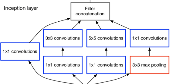
Residual NetworksExpecting over-fitting stays away; our perceptions up to this point show that raising the profundity ought to help the organization's precision. Notwithstanding, the issue with more noteworthy profundity is that it causes the sign expected to modify loads - which comes from the organization's end by contrasting ground truth and expectation - to become very little at the early layers. Basically, it shows that learning by going before levels is insignificant. It's known as an evaporating slope. The second issue with preparing further organizations is that doing so indiscriminately includes layers by endeavouring to improve a huge boundary space. This increments preparing mistakes. The remaining organizations permit the preparation of such profound organizations by developing the organization through modules called leftover models, as displayed in the figure. This is called a debasement issue. The instinct around why it works should be visible as follows: 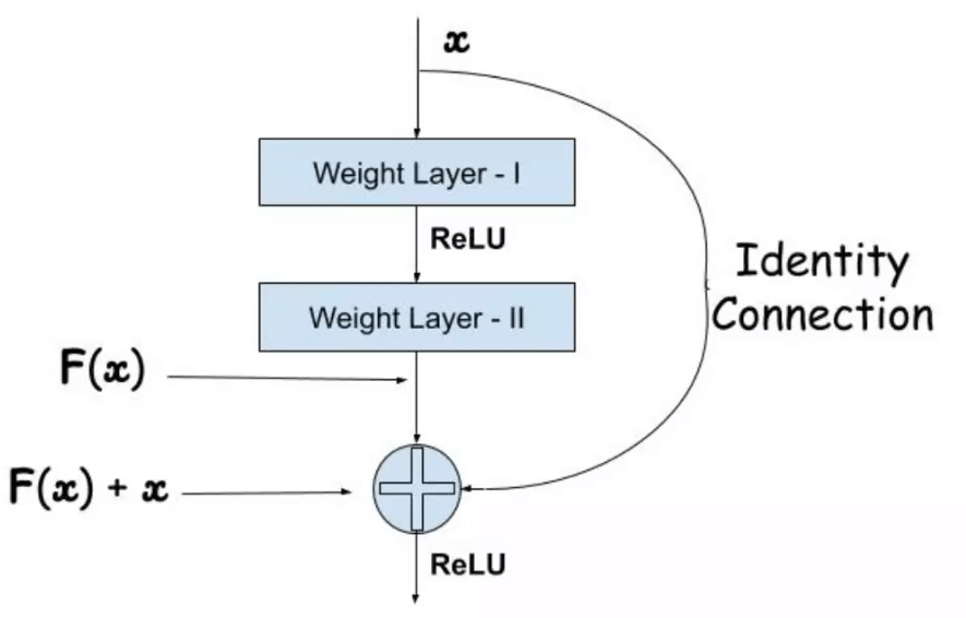
Look at network As a, which has a preparation blunder of x. Make network B by stacking extra layers on top of organization A, and afterwards, set the boundary values in those levels with the goal that the results from network An are unaffected. How about we allude to the additional layer as layer C? This would suggest that the new organization would have the equivalent x% preparing blunder. To stay away from overtraining network B, the preparation mistake ought not to be more prominent than that of organization A. Furthermore, in light of the fact that it Happens, the main clarification is that the solver doesn't prevail with regards to learning the personality planning with the additional layers-C (doing nothing to inputs and just replicating for all intents and purposes), which is definitely not a straightforward issue. To determine this, the module portrayed above lays out an immediate association between the info and result, expecting personality planning, and the extra layer-C simply has to gain proficiency with the elements on top of the information that is, as of now, open. The whole module is alluded to as the lingering module since C is just learning the remaining. It likewise utilizes worldwide normal pooling followed by the order layer, similar to GoogleNet. ResNets were learnt with network profundities as extraordinary as 152 with the upgrades illustrated. It is computationally more practical than VGGNet while accomplishing more precision than VGGNet and GoogLeNet. ResNet-152 acquires a top-five precision of 95.51. One of the tests can be utilized to assess the viability of the leftover organizations. Contrasted with the 18-layer plain organization, the plain 34-layer network showed a more noteworthy approval blunder. We currently perceive the issue as disintegration. Moreover, the indistinguishable 34-layer network has a considerably lower preparing mistake than the 18-layer remaining organization when changed into a leftover organization. 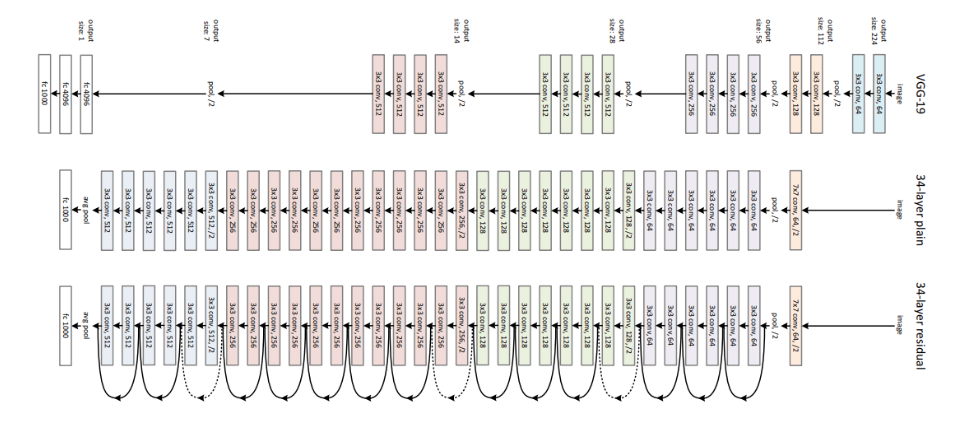
|
 For Videos Join Our Youtube Channel: Join Now
Feedback
- Send your Feedback to [email protected]
Help Others, Please Share


