| |

Rossmann Store Sales PredictionIntroduction: The demand for a good or service is constantly shifting. Without effectively predicting client demand and future sales of products/services, no firm can enhance its financial performance. Sales forecasting predicts a given product's demand or sales over a predetermined time frame. I'll demonstrate how machine learning can be used to forecast sales using a real-world business challenge from Kaggle in this post. Everything is resolved entirely from the start in this case study. So, you will watch every step of how a case study is resolved in the actual world. Issue Statement In seven European nations, Rossmann runs more than 3,000 pharmacies. Rossmann shop managers must forecast their daily sales six weeks in advance. Factors affecting store sales, including marketing, rivalry, state and federal holidays, seasonality, and location. The accuracy of the findings can be highly variable because thousands of different managers are making sales predictions based on their situations. Error Metric: RMSPE stands for Root Mean Square Percent Error. The metric's formula is as follows: 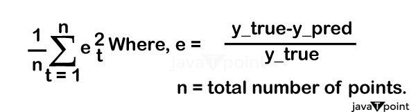
Objectives:
Data: The files are as follows:
Data fields:
StateHoliday is a flag that denotes a state holiday. With very few exceptions, all businesses are typically closed on national holidays. Keep in mind that every institution is out on weekends and federal holidays. Stands for a public holiday, B for the Easter break, C for Christmas, and N for none. If the closing of public schools impacted the ( Store, Time ), it is indicated by SchoolHoliday. StoreType distinguishes the four distinct store models ( a, b, c, and d ). Assortment - specifies three levels of assortment: basic, extra, and extended. CompetitionDistance is measuring the distance in meters to the closest rival store. CompetitionOpenSince - provides an approximation of the year and month the closest competitor was first made available. Shows whether a shop is offering a promotion that day. Promo2 is a continuous campaign that some stores are running: 0 indicates that a store is not taking part, while one indicates it is. Promo2Since[Year / Week] - specifies the calendar year and week when the store first joined Promo2. PromoInterval defines the months in which Promo2 is launched at regular intervals. Exploratory Data Analysis(EDA)Let us use EDA to obtain insights into the provided data. The following is information about train.csv: As we can see, we have around 1 million data points. Also, because this is a time-series prediction issue, we must sort the data by date. Our goal variable, in this case, is Sales. The following is information about store.csv: We have 1115 distinct shops. Many of the columns in this table have null values. We'll take charge of them in a moment. Let's look at the details of the columns in the data now. Promo: 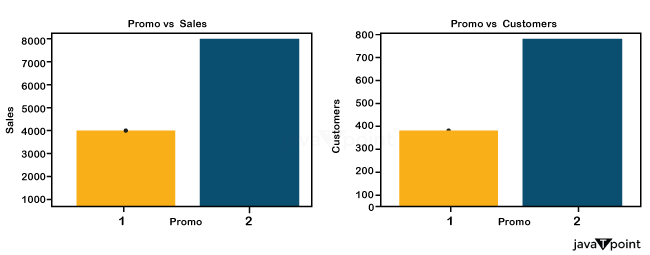
Promotion column next to Sales and Customers. We can see that revenue and consumer base increase significantly during promotions. This demonstrates that promotion has a favorable impact on a store. Sales: 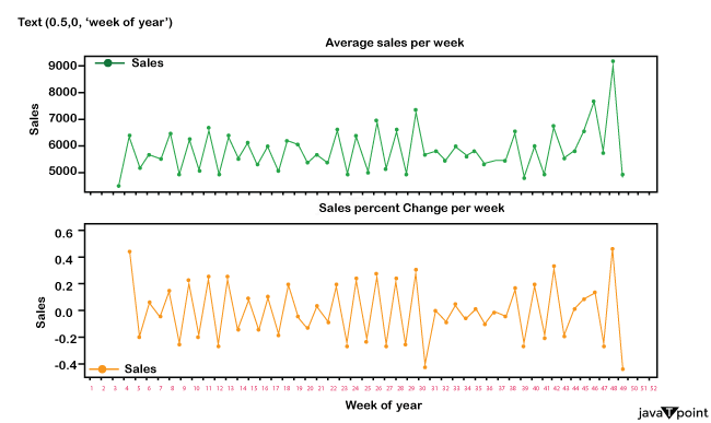
Sales over week Average It is also worth noting that Christmas and New Year's ( see graph at week 52 ) led to a spike in sales. Because Rossmann Stores offers health and beauty items, it is reasonable to assume that around the holidays and New Year's, individuals buy beauty products when they go out to celebrate, which might explain the rapid surge in sales. DayOfWeek: 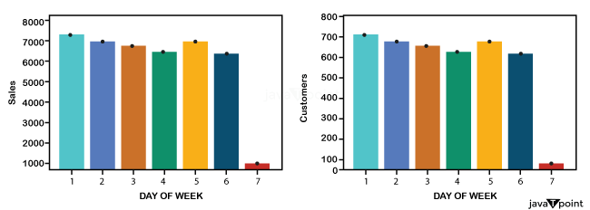
Sales and customers are compared to the DayOfWeek column. Since most stores are closed, we can see that business and consumer numbers are down on Sundays. In addition, sales on Monday are the greatest of the week. This might be because most stores are closed on Sundays. Another crucial point is that retailers operating during school vacations had more sales than usual. Customers and sales are based on a store's store type. We can see how stores of type A have a more significant number of customers and sales. StoreType D ranks second in both Sales as well as Customers. Conclusions of EDA:
Feature EngineeringOutliers Column:In this column, we will determine whether a Sales number is an outlier or not based on the Median Absolute Deviation ( MAD ). The MAD formula. We built outlier columns store per shop, which means we did it for each unique store independently and then combined the data. Date Features:First, we'll use pandas' to__datetime method to transform the Date column. Following that, we can extract further properties from Date. This week's, last week's, and next week's holidays: We've designed three features that show the total number of holidays in the current week, the previous week, and the following week. State Holiday Calculator: The function shown above was used to generate two new features. One indicates how many days remain before a state holiday, while the other shows how many days have elapsed since the last state holiday. School holiday promotion and counter: In addition to the characteristics above, I built four more that indicate the number of days before or after a promotion or a school holiday. Close dummy variable: This feature has two values: +1 or -1. +1 if the shop was closed yesterday or tomorrow; otherwise, -1. Removing data points with zeros Sales: In this case, data points with zeros are eliminated since they indicate that the store was closed for whatever reason. And if we receive a store that isn't open, we can forecast zero sales. Customers__per__day, Sales__per__customers__per__day, and Sales__per__customers__per__day: The names of the features merely indicate their meaning. There is no need for additional clarification. Open Competition and Open Promo: We are changing these two characteristics from 'year' to month as a unit. Promo interval feature generation: Promointerval is offered in the following format: May, August, November. We will split them as follows: May is one characteristic, August is another, and November is the third. Sales Variation and Acceleration: Variation = y - ( y-1 ), y = sales Acceleration equals [( y-1 ) - ( y-2 )]., where y = sales Fourier Characteristics: I use the fft function from numpy to compute Fourier frequencies and amplitudes. Then employ them as features. Other features include: These contain vital patterns about DayOfWeek, Promotions, Holidays, etc. External Information: There are just two of them for extra information. One type of data is state data, which identifies which state a shop belongs to, and the other is weather data for a particular state on a specific day. VIF Analysis: After adding all of the characteristics, we ran a VIF analysis to see whether there was any collinearity between them. High collinearity features were eliminated. Let's do some modeling right now. ModelingBase model:We used sklearn Pipe and Column Transformer to preprocess the data. The median is used to impute numerical values, whereas the most frequent is used to assume qualitative values. Numeric values are scaled as well. Now divide the data into training and validation sets. Spliting Data in test and train for OutliersOutput: Will train until test error hasn't decreased in 250 rounds. [0] train-rmspe:0.99963 test-rmspe:0.999863 [250] train-rmspe:0.41216 test-rmspe:0.487971 [500] train-rmspe:0.19972 test-rmspe:0.188309 [71] train-rmspe:1.166821 test-rmspe:1.156818 [111] train-rmspe:1.137129 test-rmspe:1.132996 151] train-rmspe:1.122311 test-rmspe:1.121135 [111] train-rmspe:1.119952 test-rmspe:1.112465 [175] train-rmspe:1.111481 test-rmspe:1.116788 [211] train-rmspe:1.193883 test-rmspe:1.112796 [251] train-rmspe:1.188571 test-rmspe:1.111461 [511] train-rmspe:1.183871 test-rmspe:1.198587 [275] train-rmspe:1.181263 test-rmspe:1.197114 [311] train-rmspe:1.177273 test-rmspe:1.195896 [351] train-rmspe:1.174326 test-rmspe:1.194886 [511] train-rmspe:1.171833 test-rmspe:1.194189 [375] train-rmspe:1.169711 test-rmspe:1.193385 [411] train-rmspe:1.167834 test-rmspe:1.192811 [451] train-rmspe:1.166113 test-rmspe:1.192347 [511] train-rmspe:1.164519 test-rmspe:1.191941 [4751] train-rmspe:1.162961 test-rmspe:1.191569 [5111] train-rmspe:1.161581 test-rmspe:1.191271 [5251] train-rmspe:1.161224 test-rmspe:1.191116 [5511] train-rmspe:1.158971 test-rmspe:1.191792 [5751] train-rmspe:1.157782 test-rmspe:1.191615 [6111] train-rmspe:1.156656 test-rmspe:1.191459 [6251] train-rmspe:1.155568 test-rmspe:1.191351 [6511] train-rmspe:1.154547 test-rmspe:1.191252 [6751] train-rmspe:1.153527 test-rmspe:1.191143 [7111] train-rmspe:1.152577 test-rmspe:1.191167 [7251] train-rmspe:1.151698 test-rmspe:1.191118 [7511] train-rmspe:1.151825 test-rmspe:1.189956 [7751] train-rmspe:1.151112 test-rmspe:1.189897 [8111] train-rmspe:1.149217 test-rmspe:1.189844 [8251] train-rmspe:1.148413 test-rmspe:1.189811 [8511] train-rmspe:1.147679 test-rmspe:1.189768 [8751] train-rmspe:1.146973 test-rmspe:1.189742 [9111] train-rmspe:1.146274 test-rmspe:1.189741 Stopping. Best iteration: [8751] train-rmspe:1.146971 test-rmspe:1.189741 Feature Selection:I did forward deciding on all of the additional features created in the feature engineering stage after generating the aforementioned basic model. The following are the new features in the pipeline: Reading store dataMeta Learning:This method is outlined as follows:
Reading sales data Output: 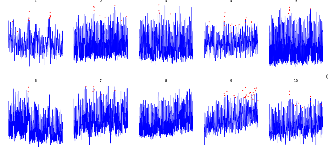
Conclusion:
Table for all scores. The table above suggests that the Light GBM Model is the best model. Future Work:With developments in Deep Learning or ML, LSTM may be an excellent place to start to enhance performance on a given dataset. Other ensemble strategies can be applied to see whether they enhance the result.
Next TopicFinding Next Greater Element in Python
|
 For Videos Join Our Youtube Channel: Join Now
Feedback
- Send your Feedback to [email protected]
Help Others, Please Share


