Diabetes Prediction Using Machine Learning

Diabetes is a medical disorder that impacts how well our body uses food as fuel. Most food we eat daily is converted to sugar, commonly known as glucose, and then discharged into the bloodstream. Our pancreas releases insulin when the blood sugar levels rise.

Diabetes can cause blood sugar levels to rise if it is not continuously and carefully managed, which raises the chance of severe side effects like heart attack and stroke. We, therefore, choose to forecast using Python machine learning.

Steps

1. Installing the Libraries
2. Importing the Dataset
3. Filling the Missing Values
4. Exploratory Data Analysis
5. Feature Engineering
6. Implementing Machine Learning Models
7. Predicting Unseen Data
8. Concluding the Report

Installing the Libraries

We first have to import the most popular Python libraries, which we will use for implementing machine learning algorithms in the first step of building the project, including Pandas, Seaborn, Matplotlib, and others.

We will use Python because it is the most adaptable and powerful programming language for data analysis purposes. In the world of software development, we also use Python.

Code

The Sklearn toolkit is incredibly practical and helpful and has practical applications. It offers a vast selection of ML models and algorithms.

Importing the Dataset

We are using the Diabetes Dataset from Kaggle for this study. The National Institute of Diabetes and Digestive and Kidney Diseases is the original source of this database.

Code

Output

<class 'pandas.core.frame.DataFrame'>
RangeIndex: 768 entries, 0 to 767
Data columns (total 9 columns):
 #   Column                    Non-Null Count  Dtype  
---  ------                    --------------  -----  
 0   Pregnancies               768 non-null    int64  
 1   Glucose                   768 non-null    int64  
 2   BloodPressure             768 non-null    int64  
 3   SkinThickness             768 non-null    int64  
 4   Insulin                   768 non-null    int64  
 5   BMI                       768 non-null    float64
 6   DiabetesPedigreeFunction  768 non-null    float64
 7   Age                       768 non-null    int64  
 8   Outcome                   768 non-null    int64  
dtypes: float64(2), int64(7)
memory usage: 54.1 KB

As we can see, all of the columns are integers, except for the BMI and DiabetesPedigreeFunction. The target variable is the labels with values of 1 and 0. A person's diabetes status is indicated by a one or a zero.

Code

Output

Filling the Missing Values

The next step is cleaning the dataset, which is a crucial step in data analysis. When modelling and making predictions, missing data can result in incorrect results.

Code

Output

Pregnancies                 0
Glucose                     0
BloodPressure               0
SkinThickness               0
Insulin                     0
BMI                         0
DiabetesPedigreeFunction    0
Age                         0
Outcome                     0
dtype: int64

We found no missing values in the dataset, yet independent features like skin thickness, insulin, blood pressure, ;and glucose each have some 0 values, which is practically impossible. A particular column's mean or median scores must be used to replace unwanted 0 values.

Code

Output

Let's now examine the data statistics.

Code

Output

Now our dataset is free of missing and unwanted values.

Exploratory Data Analysis

We will demonstrate analytics using the Seaborn GUI in this tutorial.

Correlation

Correlation is the relationship between two or more variables. Finding the important features and cleaning the dataset before we begin modelling also helps make the model efficient.

Code

Output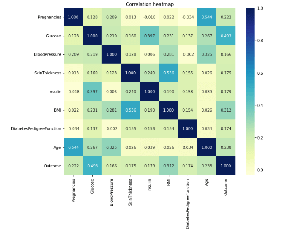

Observations show that characteristics like pregnancy, glucose, BMI, and age are more closely associated with outcomes. I demonstrated a detailed illustration of these aspects in the following phases.

Pregnancy

Code

Output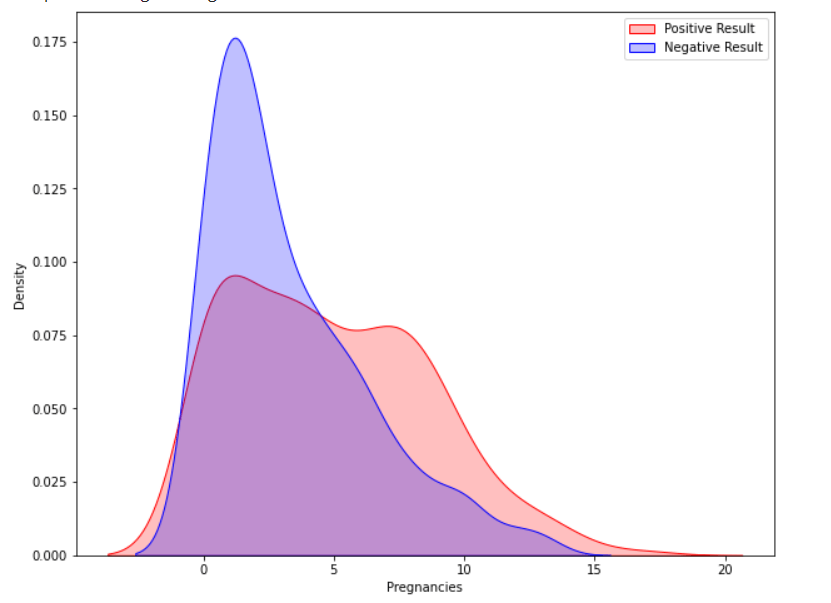

According to the data, women having diabetes have given birth to healthy infants. However, the risk for future complications can be decreased by managing diabetes. The risk of pregnancy issues, such as hypertension, depression, preterm birth, birth abnormalities, and pregnancy loss, is increased if women have uncontrolled diabetes.

Glucose

Output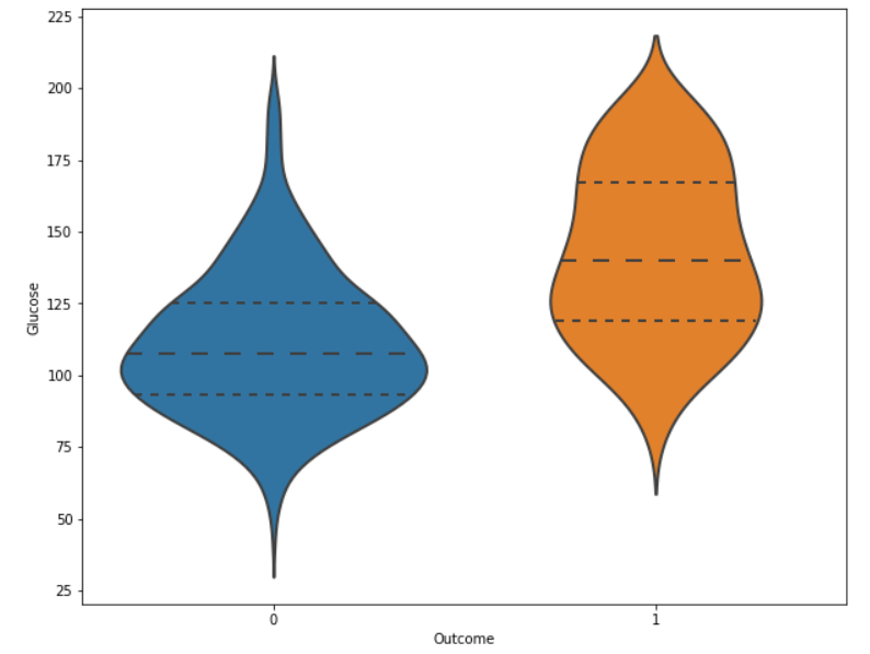

The likelihood of developing diabetes gradually climbs with glucose levels.

Code

Output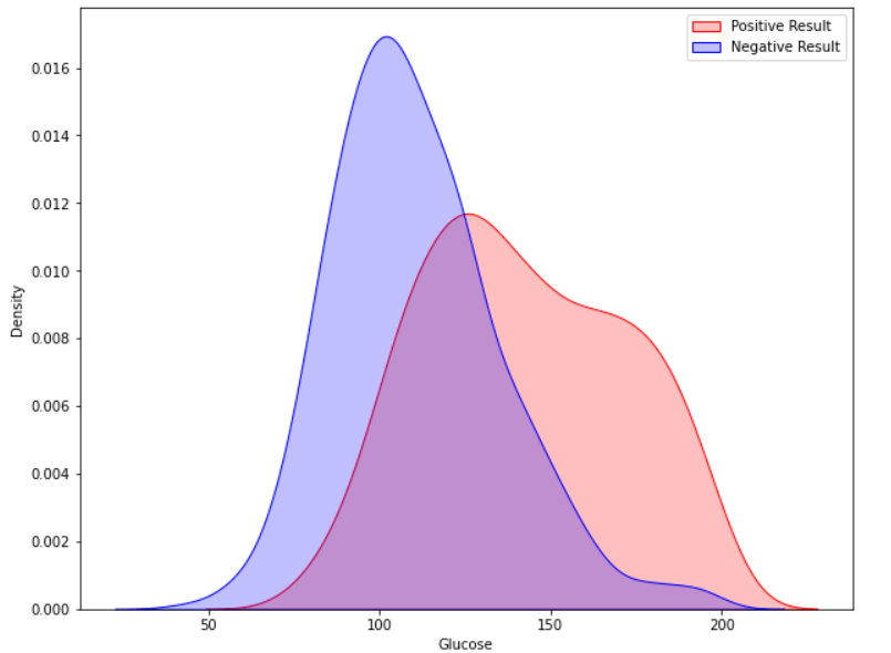

Implementing Machine Learning Models

We will test many machine learning models and compare their accuracy in this part. After that, we will tune the hyperparameters on models with good precision.

We will use sklearn.preprocessing to convert the data into quantiles before dividing the dataset.

Code

Output

Data Splitting

We will now divide the data into a training and testing dataset. We will use the training and testing datasets to train and evaluate different models. We will also perform cross-validation for multiple models before predicting the testing data.

Code

Output

The size of the training dataset:  3680
The size of the testing dataset:  2464

The above code splits the dataset into the train (70%) and test (30%) datasets.

Cross Validate Models

We will perform cross-validation of the models.

Code

A list of machine learning models is passed to the 'cv_model' function, which provides a graph of the cross-validation scores based on the mean of the accuracy values of various models supplied to the function.

Code

Output

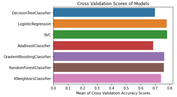
According to the above analysis, we have discovered that the RandomForestClassifier, LogisticRegression, and SVC models have higher accuracy. We will therefore perform hyperparameter tuning on these three different models.

Hyperparameter Tuning

Selecting the best collection of hyperparameters for a machine learning algorithm is known as hyperparameter tuning. A model input called a hyperparameter has its value predetermined before the learning phase even starts. Hyperparameter tuning is essential for machine learning models to work.

We have individually tuned the RandomForestClassifier, LogisticRegression, and SVC models.

Code

GridSearchCV and the classification report classes are firstly imported from the Sklearn package. The "analyse grid" method, which will display the predicted result, is then defined. We have invoked this method for each model we utilised in SearchCV. We will tune each model in the following stage.

Tuning Hyperparameters of LogisticRegression

Code

Output

Tuned hyperparameters:  {'C': 200, 'penalty': 'l2', 'solver': 'liblinear'}
Accuracy Score: 0.7715000000000001
Mean: 0.7715000000000001, Std: 0.16556796187668676 * 2, Params: {'C': 200, 'penalty': 'l2', 'solver': 'liblinear'}
The classification Report:
Mean: 0.7715000000000001, Std: 0.16556796187668676 * 2, Params: {'C': 100, 'penalty': 'l2', 'solver': 'liblinear'}
The classification Report:
Mean: 0.7675, Std: 0.16961353129983467 * 2, Params: {'C': 10, 'penalty': 'l2', 'solver': 'liblinear'}
The classification Report:
Mean: 0.7675, Std: 0.17224619008848932 * 2, Params: {'C': 1.0, 'penalty': 'l2', 'solver': 'liblinear'}
The classification Report:
Mean: 0.711, Std: 0.1888888562091475 * 2, Params: {'C': 0.01, 'penalty': 'l2', 'solver': 'liblinear'}
The classification Report:
              precision    recall  f1-score   support
           0       0.78      0.88      0.83       201
           1       0.70      0.53      0.61       107

    accuracy                           0.76       308
   macro avg       0.74      0.71      0.72       308
weighted avg       0.75      0.76      0.75       308

As we can see in the output, the best score returned by the LogisticRegression model is 0.77 with {'C': 200, 'penalty': 'l2', 'solver': 'liblinear'} parameters. Similarly, we will perform parameter tuning for other models.

Tuning Hyperparameters of SVC

Code

Output

Tuned hyperparameters:  {'C': 1.0, 'gamma': 0.0001, 'kernel': 'rbf'}
Accuracy Score: 0.7695158871629459
Mean: 0.745607333842628, Std: 0.019766615171568313 * 2, Params: {'C': 200, 'gamma': 0.0001, 'kernel': 'rbf'}
The classification Report:
Mean: 0.7521291344820756, Std: 0.02368565638376449 * 2, Params: {'C': 100, 'gamma': 0.0001, 'kernel': 'rbf'}
The classification Report:
Mean: 0.7542370483546955, Std: 0.046474062764375476 * 2, Params: {'C': 10, 'gamma': 0.0001, 'kernel': 'rbf'}
The classification Report:
Mean: 0.7695158871629459, Std: 0.016045599935252022 * 2, Params: {'C': 1.0, 'gamma': 0.0001, 'kernel': 'rbf'}
The classification Report:
Mean: 0.650001414707297, Std: 0.002707677330225552 * 2, Params: {'C': 0.01, 'gamma': 0.0001, 'kernel': 'rbf'}
The classification Report:
              precision    recall  f1-score   support

           0       0.74      0.88      0.80       201
           1       0.64      0.42      0.51       107

    accuracy                           0.72       308
   macro avg       0.69      0.65      0.66       308
weighted avg       0.71      0.72      0.70       308

SVC Model's maximum accuracy is 0.769, somewhat less than that of Logistic Regression. We can leave this model here only.

Tuning Hyperparameters of RandomForestClassifier

Code

Output

Tuned hyperparameters:  {'criterion': 'entropy', 'max_depth': 5, 'max_features': 'log2', 'n_estimators': 500}
Accuracy Score: 0.7717369776193306
Mean: 0.7673938262173556, Std: 0.0027915297477680364 * 2, Params: {'criterion': 'entropy', 'max_depth': 4, 'max_features': 'log2', 'n_estimators': 500}
The classification Report:
Mean: 0.7717369776193306, Std: 0.005382324516419591 * 2, Params: {'criterion': 'entropy', 'max_depth': 5, 'max_features': 'log2', 'n_estimators': 500}
The classification Report:
Mean: 0.7652151769798828, Std: 0.02135846347536185 * 2, Params: {'criterion': 'entropy', 'max_depth': 6, 'max_features': 'log2', 'n_estimators': 500}
The classification Report:
              precision    recall  f1-score   support

           0       0.76      0.87      0.81       201
           1       0.66      0.50      0.57       107

    accuracy                           0.74       308
   macro avg       0.71      0.68      0.69       308
weighted avg       0.73      0.74      0.73       308

Predicting Unseen Data

We have spent time working on the Exploratory Data Analysis, cross-validation of the machine learning algorithms, and hyperparameter tuning to identify the best model that fits my dataset. We will now make predictions using the model of tuned hyperparameters with the highest accuracy score.

Code

Output

precision    recall  f1-score   support

           0       0.78      0.88      0.83       201
           1       0.70      0.53      0.61       107

    accuracy                           0.76       308
   macro avg       0.74      0.71      0.72       308
weighted avg       0.75      0.76      0.75       308

Finally, append a new feature column in the test dataset called Prediction and print the dataset.

Code

Output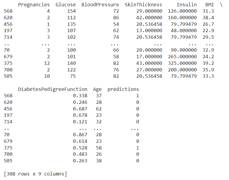

Concluding The Report

1. One of the risks during pregnancy is diabetes. It will have to be diagnosed to avoid problems.
2. An increase in glucose levels is strongly correlated to a rise in diabetes.
3. Logistic Regression with tuned parameters has given the maximum accuracy score.