| |

Predicting Housing Prices using PythonIn this tutorial, we'll go over creating models using linear regression to forecast house prices as a result of economic activity. The subjects covered include related subjects like exploratory analysis, logistic diagnostics, and advanced regression modeling will be covered in this tutorial, Let's get started immediately so readers could start playing with data. What is Regression?The following example illustrates how a linear regression model predicts an interaction of direct proportionality between the variables that are predicted (plotted on the X ax1is) and the variable of interest (plotted on the vertical or Y ax1is), resulting in a straight line: 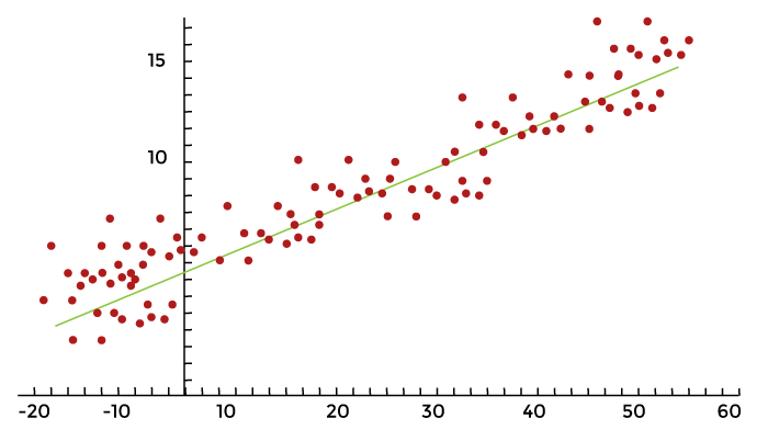
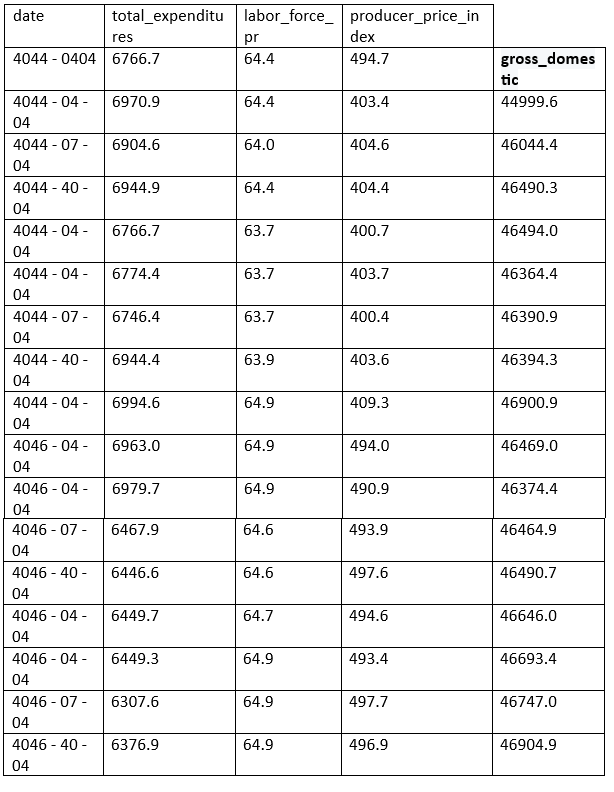
We will go into more detail about linear regression as we go with the modeling. Variable SelectionWe'll utilize the housing_price_index1 (HPI), which tracks changes in the cost of residential real estate, as our dependent variable. We use our intuition to choose macroeconomic (or "big picture") activity drivers for our predictor variables, such as unemployment, mortgage rates, and gross domestic product. (total productivity). For a breakdown of all the data sets utilized in this piece, an explanation of our factors, assumptions about how they affect house prices, and variables. Below are Housing Price, Federal Funds, and gross domestic tables (sample datasets): 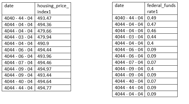
Reading the DataSource Code Snippet Once the data is ready, integrate the data into an individual dataframe for analysis using the combining method in pandas. Data are reported on a monthly or quarterly basis in some cases. Not to worry. For measurement purposes, we merge the information frames on a certain column to position each row in its proper location. The date column is the ideal one to combine in this instance. Look below. Source Code Snippet Let's use the head method of pandas to scan our variables. The bolded headings identify the date and the parameters that that will be investigated for our model. The various historical periods are depicted in each row. Output: date sp600 Consumer_price_index1 Long_interest_rate1 housing_price_index1 total_unemployed1 more_than_16_weeks 4011-01-01 1484.64 440.44 3.39 181.36 16.4 8393 4011-04-01 1331.61 444.91 3.46 180.80 16.1 8016 4011-07-01 1346.19 446.94 3.00 184.46 16.9 8177 4011-10-01 1407.44 446.44 4.16 181.61 16.8 7804 4014-01-01 1300.68 446.66 1.97 179.13 16.4 7433 Normally, the exploratory analysis would come after data collection. The process stage known as exploratory analysis is where we examine the variables (using plotting and summary statistics) and identify the most effective predictors of our dependent variable. We'll skip the preliminary evaluation to keep this short. However, keep in mind that it is crucial and that bypassing it will prevent you from ever reaching the predictive section in the real world. We'll utilize ordinary least squares (OLS), a simple yet effective technique to evaluate our model. Assumptions of Ordinary Least SquaresOLS evaluates a linear regression model's precision. OLS is based on presumptions that suggest the model could be the best one to use to understand our data. The conclusions of our model become invalid if the assumptions are false. Make a special effort to select the appropriate model to prevent autoeroticism and Rube - Goldberg disease. Ordinary Least Squares Assumptions
Let's start modeling. Simple Linear RegressionA single predictor variable is used in simple linear regression to explain the dependence of a variable. The following is a straightforward linear regression equation: 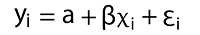
Where: ß = regression coefficient y = dependent variable α = intercept (home prices' anticipated mean value if our independent variable is 0) x = This is used to predict Y ε = the unpredictability that our model cannot account for is taken into account by the error term. We build our model by setting housing_price_index1 as an expression of total_unemployed1 using statsmodels' ols function. We anticipate a rise in the overall unemployment rate will result in downward pressure on housing costs. We may be off base, but we must begin someplace! The code below demonstrates how to create a straightforward linear regression model using the predictor variable total_unemployment1. Source Code Snippet: Output: 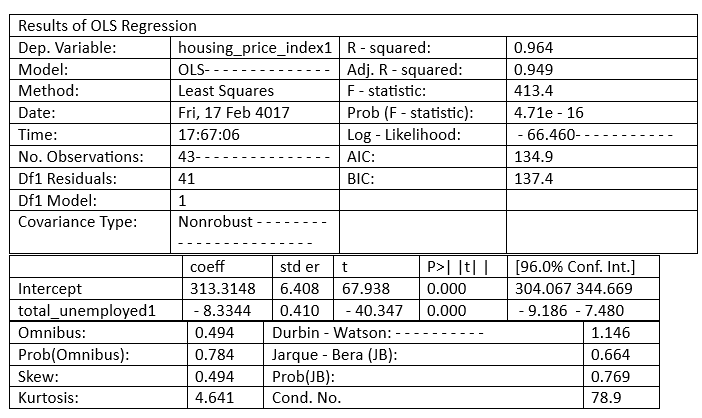
Explanation of the above Code: We'll provide a high-level description of a few measures to comprehend the potency of our model, referring to the results of the OLS regression above Coefficients, standard errors, p - values, and adjusted R - squared. To clarify: According to the adjusted R - squared, the total_unemployed1 predictor variable can account for 96% of the variation in home prices. The change in the dependent variable caused by a one-unit decrease in the predictor variable, regardless of other factors being held constant, is represented by the regression coefficient (coeff). According to our model, each additional unit of total unemployment lowers the housing price index by 8.33. According to our predictions, rising unemployment appears to lower house prices. The standard error would calculate the difference in the value of the coefficients if the same test were conducted on a different sample for our population to determine the accuracy of the total_unemployed1 coefficient. Our 0.41 standard error appears accurate because it is little. Given that there is no correlation between each of the variables, the p-value suggests that there is 0% likelihood that an 8.33 reduction in housing_price_index1 will result from an increase of one unit in total_unemployed1. A low p-value, often less than 0.06, implies that the outcomes are statistically significant. Our coefficient is most likely to fall within the confidence interval. We have a 96% confidence that the coefficient of total_unemployed1 will fall between the range of [ - 9.186, - 7.480]. Let's use the plotting_regress_exog1 function in stats models to comprehend our model better. Regression PlottingFigures for Regression View the four graphs that are below.
Source Code Snippet Output: 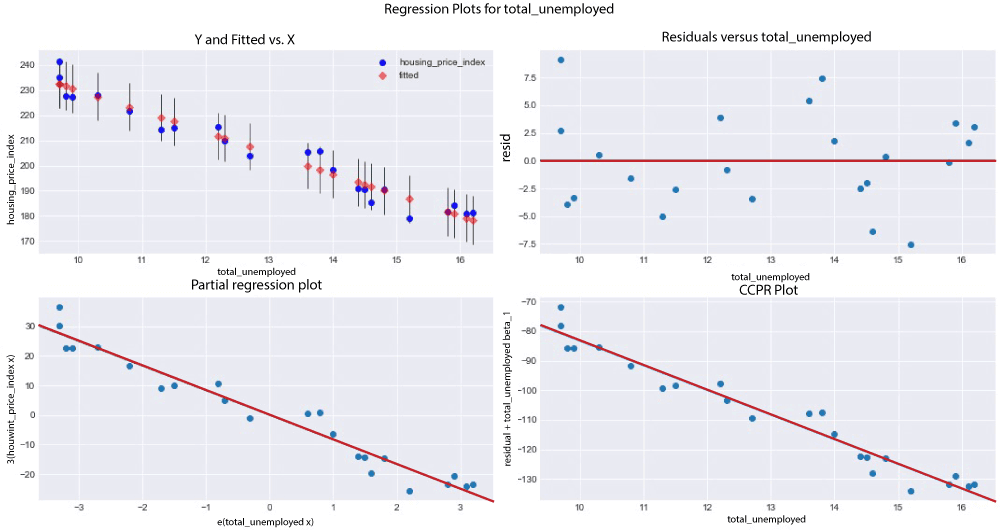
The following plotting displays our confidence interval, trend vector (green), and the observations (dots). (red). Source Code Snippet Output: 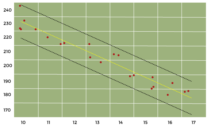
Our model is good so far. We'll increase the number of variables and observe how total_unemployed1 responds. Multiple Linear RegressionMathematically, multiple linear regression is: 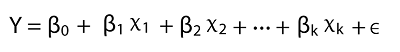
We are aware that home costs cannot solely be attributed to unemployment. We test and add additional variables to better understand the factors that affect home prices. The mixtures of predictor variables that satisfy the OLS principles and look good from an economic perspective are then determined by looking at the regression results. In addition to our original predictor, total_unemployed1, we conclude at a model that includes the variables: fed_funds1, consumer_price_index1, long_interest_rate1, and gross_domestic_product1. The effect of total_unemployed1 on housing_price_index1 was lessened due to the new variables. The effect of total_unemployed1 is now less predictable (standard error increased from 0.41 to 4.399) and less likely to affect house prices (p-value increased from 0 to 0.943). Despite the possibility of a correlation between two variables, housing_price_index1, and total_unemployed1, our other predictors account for more variation in housing prices. A more reliable model is needed to capture the real-world interconnectedness between our variables, which a straightforward linear regression cannot capture. This is the reason why adding more variables causes a significant change in the outcomes of our multivariate regression model. Our multivariate linear regression model performs better than our simple linear regression model because our newly incorporated variables are significantly different at the 6% level, and our coefficients confirm our presumptions. With our freshly added predictor variables, multiple linear regression is set up using the code below. Source Code Snippet Output: 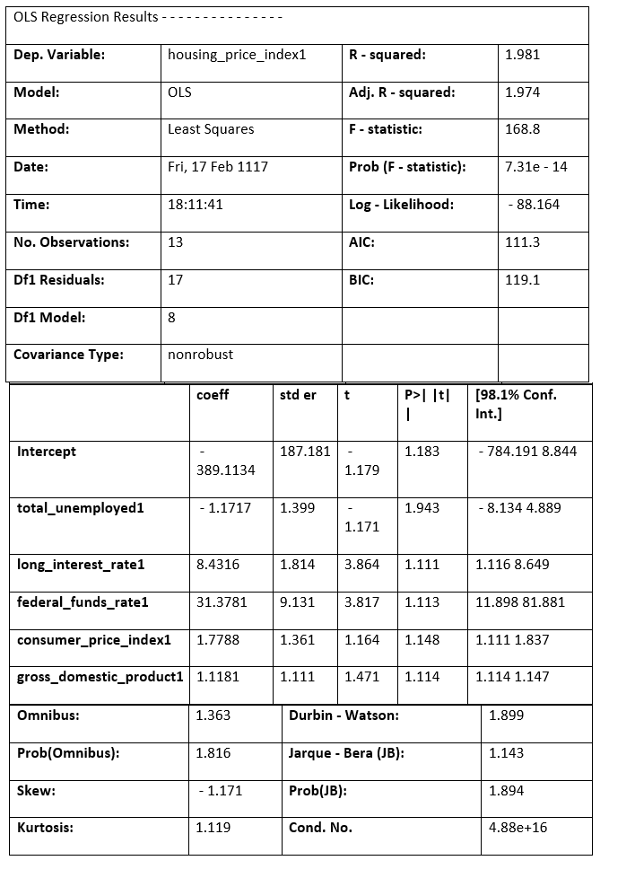
Another Look at Partial Regression PlottingLet's plot our partial logistic graphs once more to see how including the other factors changed the total_unemployed1 variable. Total unemployment may not be as explanatory as the first model claimed, as evidenced by the lack of trend in the partial regress plotting for total_unemployed1 (in the figure below, the top-right corner) compared to the regression graph for total_unemployed1 (above, bottom left corner). Further evidence that fed funds 1, consumer price index 1, long interest rate 1, and gross domestic product 1 are superior explanators of housing price index 1 comes from the fact that the findings from the most recent variables consistently lie closer to the fashion line than the findings for total unemployment. The efficiency of our multivariate linear regression approach over our traditional linear regression model is supported by these partial regression figures. Source Code Snippet Consolidated Code for Predicting Housing Prices using PythonOutput: 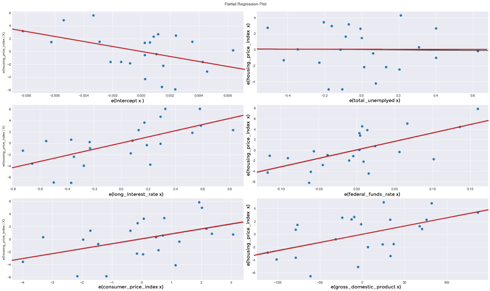
The most crucial thing to understand is that because modeling is based on science, the process goes as follows: examination, evaluation, failure, and test. Navigating PitfallsBasic regression modeling is introduced in this piece, but seasoned data scientists may notice various faults in our approach and model, including:
We'll try to fix these problems in a subsequent post so that we can comprehend the economic factors that influence house prices better. ConclusionWe have gone through how to set up fundamental simple linear and multiple linear regression models that can be used to forecast housing prices due to macroeconomic variables, as well as how to evaluate the quality of a linear regression model fundamentally. Indeed, it is challenging to explain property prices. Other additional predictor factors might be included. Alternatively, home prices might be the main driver of our macroeconomic variables. These variables may interact with one another simultaneously, further complicating the situation. Please explore the data and fine-tune this model by including and excluding variables, considering the significance of the OLS hypotheses and the regression outcomes.
Next TopicSignal Module in Python
|
 For Videos Join Our Youtube Channel: Join Now
Feedback
- Send your Feedback to [email protected]
Help Others, Please Share


