| |

How to Draw the Mandelbrot Set in PythonThis tutorial will discuss about an interesting project that involves complicated numbers by using Python. We will learn about fractals and make incredible artwork using an illustration of the Mandelbrot Set with Python's Matplotlib and Pillow libraries. We will also find out the process by which this fractal was created and its significance, and how it is related to other fractals. Understanding the concept of object-oriented programming principles and the concept of recursion will allow us to make the most of Python's expressive syntax and write simple code that reads as math formulas. To comprehend the algorithms of creating fractals, we need to be comfortable working with complicated mathematical concepts like logarithms, set theory, and repeated functions. However, don't let these basics be a hindrance, as we will be able to follow along and make the art however you like! How to Understand the Mandelbrot SetBefore we attempt to draw the fractal, we need to know the Mandelbrot set and how to identify its members. If we are already acquainted with the basic theory, then we are free to proceed to the part of plotting below. The Icon of Fractal GeometryIf the name isn't familiar to the user personally, they may have seen some stunning visualizations that are part of the Mandelbrot set prior to that. It's a collection of complicated numbers which form an intricate and distinctive pattern when shown on the intricate plane. This pattern was probably the most famous fractal and gave birth to the concept of fractal geometry in the latter half of the 20th century. 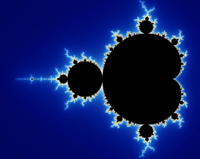
Mandelbrot set was made possible because of the advancements in technology. It's believed to be the work of a mathematician called Benoit Mandelbrot. He worked for IBM and was able to access computers that could do what was back then, a plethora of numbers crunching. Nowadays, it is possible to look into the fractals from the comfort of our home using only Python! This discovery, Mandelbrot's set, was made possible by technological advancement. Fractals are endlessly repeating patterns that occur in various sizes. Philosophers have debated the existence of the infinite for many centuries, and fractals have a parallel in our world. It's an extremely regular phenomenon that occurs in the natural world. For instance, this Romanesco cauliflower is not infinite but is a self-similar form because every part of the plant appears like the whole, just smaller. 
Self-similarity is often defined mathematically using the notion of recursion. Indeed, the Mandelbrot set isn't self-similar in the sense that it is since it is composed of two slightly different versions of the set at smaller dimensions. Yet, it can be described as a recursive function within the complex domain. The Boundary of Iterative StabilityThe Mandelbrot set refers to the collection of complex numbers called c. The infinite number of sequences, such as z0, z1, ..., zn, ..., remains bounded. Also, an upper limit to the size of any number complex within that sequence is never greater than. The following formula for recursive defines this Mandelbrot sequence: 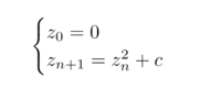
In simple English, in order to determine whether some complex number, c, is part of the Mandelbrot set, we need to feed that number into the formula below. The number we input will remain the same as we go through the sequence from this point on. The initial element of this sequence, the number z0, will always be the same as zero. To calculate the following element zn+1, we will continue by squaring the previous element, zn. Then, we will be adding the beginning number, which is c, to create the feedback loop. In observing how the sequence of numbers of functions and how it behaves, we will be able to categorize the complex numbers, c, as either a Mandelbrot set or not. The choice to make is arbitrarily based on the level we have set for certainty since more components can provide a precise conclusion on the number of c. The sequence is infinitely long. However, we have to end calculating its elements at the point we are able to stop. For complex numbers, we could visualize this process in two dimensions. However, it would be best if we looked at only the real numbers for the simplicity of the process now. Should we decide to apply the equation above in Python, it would be something like this: Our z() function returns the nth element of your sequence. This is the reason it will take the index of an element, n, as the first argument. The second argument, "c," can be regarded as a fixed number you're trying to test. The function will continue to call itself indefinitely because of the recursion. To break the chain of repeated calls, A conditional check on the basic case using an immediate solution known as--zero. Test our new formula to determine the ten first elements of this sequence for the formula c = 1 and observe what happens: Output: z(0) = 0 z(1) = 1 z(2) = 2 z(3) = 5 z(4) = 26 z(5) = 677 z(6) = 458330 z(7) = 210066388901 z(8) = 44127887745906175987802 z(9) = 1947270476915296449559703445493848930452791205 Note the rapid increase in these sequence components. It reveals something about the composition in the c 1. Particularly this has to fit into the Mandelbrot set because the sequence it's based on is not bound. Sometimes an iterative method may be more effective than a recursive method. Here's an alternative function that produces an infinite sequence with the input value specified c: Sequence() functions return a sequence of elements. sequence() function returns a Generator object giving successive components of the series indefinitely through the form of a loop. Since it doesn't provide the indices of the elements that you could identify them and then stop it after a certain number of iterations. Output: z(0) = 0 z(1) = 1 z(2) = 2 z(3) = 5 z(4) = 26 z(5) = 677 z(6) = 458330 z(7) = 210066388901 z(8) = 44127887745906175987802 z(9) = 1947270476915296449559703445493848930452791205 The results are identical to the previous version. However, the generator function allows us to determine the sequence elements with greater efficiency through an algorithm that is lazy in its evaluation. Additionally, iteration eliminates redundant function calls that require the already computed sequence elements. This means that we are not in a chance of exceeding the maximum number of recursion elements in the future. The majority of numbers cause this sequence to diverge until infinity. But, some will make the sequence steady by converging the sequence to one value or remaining within a certain interval. Some will ensure that the sequence is continuously stable by alternating back and across the same values. Stable and regularly stable values comprise what is known as the Mandelbrot set. For instance, adding an integer c = 1 will make the sequence expand without limit as you've learned it. However, the value c = -1 causes it to jump between 0 and 1 frequently, whereas the combination c = 0 results in the sequence with only one number:
It's difficult to determine the numbers that can be considered stable and those that aren't since it is virtually insensitive even to one tiny change in the value that was tested c. If we place the solid numbers in the complicated plane, then we will observe the following pattern appear: 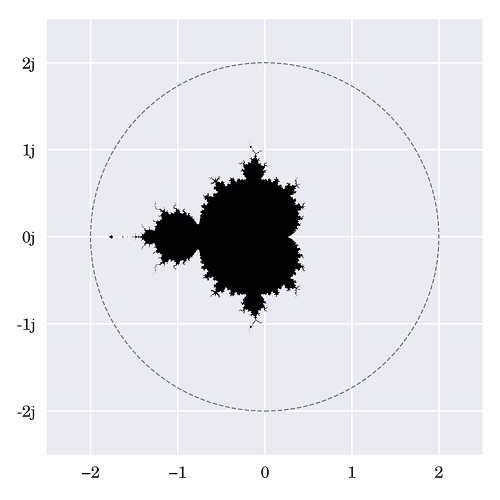
The image was created by using the recursive formula at least 20 times per pixel, each pixel representing a number of values. If it were determined that the value of the resultant complex number remained tiny after all the iterations, then the corresponding pixel would be colour-black. However, when the magnitude was larger than the radius of two, the process ended and skipped the present pixels. It may be surprising that a simple formula that only requires multiplication and addition can create an intricate structure. But it's not the only thing. It's been discovered that we can use this formula and apply it to create endlessly different Fractals. The Map of Julia SetsIt isn't easy to talk about this set without also mentioning the Mandelbrot set without also mentioning the Julia sets that were found in the work of French mathematician Gaston Julia several decades before without the assistance of computers. Julia sets, as well as sets of the Mandelbrot set, are very closely linked since they can be obtained using the same formula but with different sets of start conditions. There is just one Mandelbrot set; there are many Julia sets. We started the sequence with the z0 = 0 in the past. We will then systematically check some arbitrarily intricate number, for example, c, to determine if it was a member. In contrast, in order to determine whether a given number belongs to a Julia sequence, we have to select that number as the point of departure for the sequence and then select a different number as the c parameter. Here's a quick overview of the formula's definitions based on the set we are studying:
In the first instance, c represents a possible member of the Mandelbrot Set and is the sole input value needed since Z0 remains set at zero. But every term alters its meaning when using that formula while when we are in Julia mode. In this case, c works as a parameter that determines the form and shape of the whole Julia set, and the value z0 will become our primary focus. As before, the formula for a Julia set requires only two input values. We could modify a function we have previously defined so that it becomes more general. This will allow us to create infinite sequences that begin from any point instead of always zero. Because of this default value of the argument highlighted in this line, we can still utilize this function just in the same way as before since the z is not required. In addition, we can alter the point at which we begin the sequence. We might get more clarity after we have defined function wrappers for Mandelbrot or Julia sets: Every function will return an object generator tuned to our preferred starting condition. The principles used to determine whether an individual value is part of the Julia set are similar to the Mandelbrot set you observed earlier. In short, we need to repeat the process and then observe its evolution over time. Benoit Mandelbrot was studying Julia sets during his research. Particularly interested was locating the values of the c, which result in so-called Connected Julia sets, as opposed to their unconnected counterparts. These are referred to by the name of Fatou sets and are characterized as dust composed of an innumerable amount of fragments when viewed on the plane of the complex: 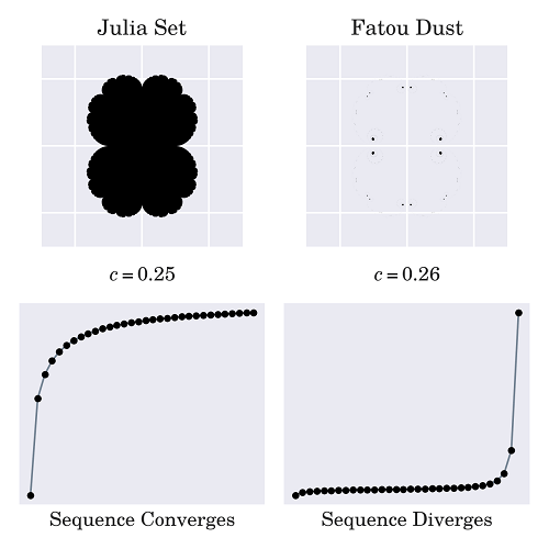
It is well-known that plugging any member of the Mandelbrot set into the formula for recursive will result in a series of complex numbers that will converge. The image at the top-left corner shows a connected Julia set derived from the formula c = 0.25, which is part of the Mandelbrot set. The numbers are converged up to 0.5 in this instance. A slight alteration to the number c could turn your Julia set into dust and cause the sequence to split infinity. The connected Julia sets are correlated to the c values that produce stable sequences using the formula for recursive above. We could claim the idea that Benoit Mandelbrot was looking for the boundary that would allow iterative stability or a map of all Julia sets, which would reveal the places where these sets are connected and also where they're not. Plotting the Mandelbrot Set Using Python's MatplotlibThere are a variety of ways to display the Mandelbrot set using Python. They can be used to avoid needing to convert between world coordinates and the pixels coordinates. If the users are familiar with working with the NumPy library as well as Matplotlib, The two libraries in combination will offer one of the easiest methods to visualize the fractured. To create the initial list of candidates, we can make use of np.linspace() that creates evenly spaced numbers within the specified range: The function described above will produce an array of two-dimensional complex numbers enclosed in the rectangular space defined with four variables. These parameters are the x_min as well as the x_max parameters that determine the boundaries of the horizontal direction. In contrast, the y_min and y_max are the same with regard to the vertical. The fifth parameter, the pixel density, is the one that determines the number of pixels per unit. We can now use this array composed of complicated numbers and use the well-known formula for recursive computation to determine which numbers are stable and those that don't. Because of the NumPy's vectorization, the matrix can be passed to the matrix as one element, c, and then perform calculations for each element without writing explicit loops: The code that is highlighted on the line is executed for the entire elements of matrix c during each repetition. Since Z and c begin with different dimensions at first, NumPy uses broadcasting to extend the latter so that they have the same forms. The function creates a 2D image consisting of Boolean values on the resulting array, z. Each value is correlated to the stability of the sequence at this time. To benefit from vectorized computation, the loop in this code continues adding and squaring numbers indefinitely regardless of how large they were already. This isn't ideal since it is common for the numbers to begin to diverge very early, which makes the majority of the calculations inefficient. Additionally, the numbers that rise rapidly can result in an error due to an overflow. NumPy detects overflows causing problems and warns users in the standard error stream (stderr). If we would prefer to block these warnings, we can set up a filter prior to using your program: After a set number of iterations, the magnitude of each number in the matrix will remain within or go over that threshold by two. If they are not, they will likely be members of the Mandelbrot set. They can be visualized with Matplotlib. Low-Resolution Scatter PlotA simple and easy method of visualizing the Mandelbrot set is to use the use of a scatterplot which shows the relationship between variables. Since complex numbers are a combination of physical or real and imaginary components, breaking them up into separate arrays is a good fit using the scatter plot. First, we must transform a Boolean security mask into complex numbers that create the sequence. We can do this using NumPy's masking filtering: This function returns a one-dimensional array that consists of only those complex numbers which are stable and thus belong to the Mandelbrot group. If our functions are described in the previous section, we will be able to create a scatter plot with Matplotlib. Make sure to include the import statement we need at the top of the file. This will bring the plotting interface to the current namespace. We can now calculate our information and plot it: The method of complex_matrix() prepares a rectangular array of complex numbers that span the range from -1.5 to 0.25 on the x-direction. It is within -2 as well as 2 in the direction of y. The following operation for find_members() passes through only the numbers part of the Mandelbrot set. Then, plot.scatter() plots the set in addition, plot.show() will reveal this picture: 
This is a re-enactment of mathematical history! It's 749 points long and is akin to an original ASCII printout created using dot matrix printers by Benoit Mandelbrot himself a few years ago. We can play around with the pixel density and our number of repetitions to determine how they affect the final result. High-Resolution Black-and-White VisualizationFor a more precise visualization of the Mandelbrot plot in white and black, we can increase the number of pixels on our scattering plot until individual dots are difficult to distinguish. Using the binary colormap to create the Boolean stabilization mask, we can also use the Matplotlib plot.imshow() function. Just a handful of changes required in your current code: Make sure we increase our pixel density to a high value, like 612. After that, we can remove any callback to the function get_members() and replace the scatter plot with plot.imshow() to display the data in an image. If all goes as planned, we should be able to look at this image in Mandelbrot's set: Mandelbrot set: 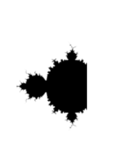
To narrow down on the part of the fractal, alter the boundaries for the matrix in that area as well as increase the frequency of the iterations to a ratio of 10 or more. It is also possible to experiment with various colormaps made available by Matplotlib. But, to let our creativity flow, we might want to experiment by using Pillow, one of Python's most popular imaging libraries. ConclusionWe now know how Python can be used to plot and draw the famous Benoit Mandelbrot fractal. There are many ways to visualize it using colors, grayscale, black and white, and other visualizations. A practical example has been shown to show how Python can elegantly express complex mathematical formulas. In this tutorial, we have learned how to:
Next TopicPython Dbm Module
|
 For Videos Join Our Youtube Channel: Join Now
Feedback
- Send your Feedback to [email protected]
Help Others, Please Share


