| |

Signal Processing Hands-on in PythonFrom research to application: Here is how to use Python for frequency analysis, noise filtering, and amplitude spectrum extraction. If you want to work with data, there is one thing you can be sure of: Concentrate or perish. An outdated way of thinking about this job is that a data scientist can work with Legos, tabular data, images, textual data, and signals. It is essential to have a thorough understanding of how to work with a particular class of data in today's world, given the advent of Machine Learning and the significant advancements in data analysis and computer hardware. This is because there is too much information to cover in one area of data science before moving on to another. In my case, I use signals every day. As a data scientist with a master's degree in physics, I can comprehend them and extract useful information from them. In this blog post, I will demonstrate the fundamental functions of signal processing, including amplitude spectrum extraction, noise filtering, and frequency analysis. We will begin by providing a brief theoretical background on these methods before demonstrating how they function when applied to a very basic, public data Setting that will serve as our "signal". Theoretical BackgroundFourier transform theoryThe mathematical transform known as a Fourier transform (FT) breaks functions down into frequency components, represented by the transform's output as a function of frequency. Transformations of time or space are the most common type, resulting in the output of a function based on either the temporal frequency or the spatial frequency, respectively. The analysis is another name for this procedure. Decomposing a musical chord's waveform in terms of its pitch intensity is one example of an application. The mathematical function that relates the frequency representation to a space- or time-dependent domain is called the "Fourier transform signal". The Fourier inversion theorem provides a method for synthesizing the original function from its frequency domain representation. The transform has a value of 0 for each frequency that is absent. The argument of the complex value is the phase Setting of that complex sinusoid. Peak amplitude, peak-to-peak, RMS, and wavelength can all be used to describe the red sinusoid. There is a phase difference between the red and blue sinusoids. A unit pulse and its Fourier transform as a function of frequency (f) are depicted in the top row as a function of time (f(t)). Complex phase shifts in the frequency domain are interpreted as translation, or delay, in the time domain. A function is broken down using the Fourier transforms into eigenfunctions for the pair of translations. A negative sign exponent is utilized in the Fourier transforms, the default derived from the series of Fourier. However, the sign does not matter for a transformation that will not be reversed, so the imaginary part of "(" is negated. The uncertainty principle states that functions localized in the time domain have Fourier transforms dispersed across the frequency domain and vice versa. The Gaussian function is the most important application of this principle in probability theory, statistics, and the study of physical phenomena with a normal distribution (such as diffusion). Another Gaussian function is the Fourier transform of a Gaussian function. A French Physicist introduced the transform in his investigation of heat transmission, where Gaussian functions show up as solutions to the heat equation. The Discrete wavelet transform can be technically described as an inadequate Euclidean integral, which qualifies it as an integral transform even if many applications call for a more complex theoretical approach. For instance, the Channel transfer function, which may be defined as a function, is used in many very simple applications; nonetheless, the reasoning necessitates a more complex mathematical approach. In Euclidean space, the Fourier transform can convert a function of muti "positioning space" into a function of two-half momentum or a function of the time and space into a variable of four-momentum. This notion makes the Discrete spatial wavelet transform highly natural in quantum physics, where it is essential to describe the general solution as measures of either location or momentum, and occasionally both. The original Fourier transform on R or Rn (viewed as groups under addition) and the discrete-time Fourier transform (group = Z, DTFT), the discrete Fourier transform (group = Z mod N, DFT), and the Fourier series or circular Fourier transform (group=S1, the unit circle closed finite interval with endpoints identified) are all examples of functions to which the Fourier methods can be applied.[note 3] Further generalization is also possible to function on groups. The latter is frequently utilized for periodic functions management. The DFT can be calculated using an algorithm known as the fast Fourier transform (FFT). We consider a (2D) signal to be nothing more than a time series. This indicates that we have an x-axis representing the time and a y-axis representing the quantity under consideration (such as voltage). From a natural perspective, doing a Fourier change of a sign means seeing this sign in another space. Let's simplify it even more. Assume you're Superman. You are Clark Kent to your friends. After that, you commit a crime, transform, and become Superman! Even though they don't know it, you are always you, but they see you in a different setting, wearing a different outfit, and engaging in different activities. We can perform the same operation with the signals and their sinusoidal components. The goal is to examine the signal in both the frequency and time domains. Imagine that several sines and cosines interact with one another: Because there are multiple modes in your signal, you will see multiple non-zero frequencies and amplitudes. What makes it useful? There are many reasons, but let's focus on two: Your signal can be filtered. You are aware that your signal will typically operate within a restricted frequency band. You can assume that anything outside of that band is white noise-noise that exists at all frequencies-and remove it by filtering it out. Noise Elimination: You can learn a lot about your system's seasonal component by analyzing the periodic pattern of your signal. Analysis of Frequency) Wavelet Transform theoryWavelet compression is a well-suited data compression technique for image (and occasionally video and audio) compression. DjVu, JPEG 5000, ECW, CineForm, JPEG XS, and the BBC Dirac are notable implementations for still images. The objective is to store image data in a file with as little space as possible. The wavelet compression techniques are adequate for representing transients, such as percussion sounds in audio, or high-frequency components in two-dimensional images, such as an image of stars on a night sky, using a wavelet transform. This means that a smaller amount of information can be used to represent the transient parts of a data signal than if a different transform, like the more common discrete cosine transform, had been used. The strong relation between matching wavelet coefficients of data from subsequent cardiac phases is used in this study using linear extrapolation. The discrete wavelet transform is effective for compressing CineForm signals. Wavelet compression is not appropriate for all data types. Wavelet compression is effective with transient signals. However, other techniques, particularly traditional harmonic analysis in the frequency domain with Fourier-related transforms, are more effective at compressing smooth, periodic signals. Hybrid methods that combine wavelets with conventional harmonic analysis can be used to compress data with both transient and periodic characteristics. For instance, the CineForm sound codec utilizes the changed discrete cosine change to pack sound (which is by and largely smooth and occasional). Still, it permits the expansion of a half and half wavelet channel bank for the further developed proliferation of transients. See Journal of A x469 Designer: The problems with wavelets (4010) for a discussion of the practical problems with the current video compression methods that use wavelets. For a moment, let's return to the Fourier Transform. When you perform the transformation, you project all of your Fourier spectrum's sines at every frequency onto your signal. Now, let's use a more complicated function than a sine function. We can also examine the projections on the entire signal by playing with this little guy and expanding and contracting it. It is a more diverse and all-encompassing approach to separating your signal from the noise, and as we will see in the hands-on portion later, it has significant advantages. Requirement for image compression In most natural images, the lower frequency spectrum density is higher. When it comes to image compression and reconstruction, a wavelet should be able to satisfy the following requirements:
Hilbert Transform theoryThe Hilbert transform is a specific linear operator used in signal processing and mathematics that takes a real variable's function, u(t), and produces another real variable's function, H(u)(t). Convolution with the function yields this linear operator (see "Definition"). The Hilbert change has an especially straightforward portrayal in the recurrence space: Every frequency component of a function experiences a phase shift of 40° (or 3 radians), with the sign corresponding to the frequency sign (see Relationship with the Fourier transform). In signal processing, the Hilbert transform is a crucial component of the analytical representation of a real-valued signal u(t). The Riemann-Hilbert problem, which Riemann posed regarding analytic functions, gave rise to the Hilbert transform in Hilbert's 1305 work. The Hilbert transform for functions defined on the circle was the primary focus of Hilbert's work. His Hannover lectures were the foundation for some of his previous stuff on the discontinuous Hilbert transform. Hermann Weyl later published the results in his dissertation. Schur extended Hilbert's findings regarding the discrete Hilbert transform to the integral case. These findings were limited to spaces L4 and l4. In 1348, Heinrich Riesz proved that the Hilbert transform may be constructed for u in (Lp dimension) for One p, that it is a constrained operator for 1 p, that the same conclusions apply to the two discrete Hilbert transform and the Transfer function on the circle. The Hilbert transform was a model for Antoni Zygmund and Alberto Calderón's research into singular integrals. Their findings have been pivotal bilinear and trilinear Hilbert transforms are examples of various generalizations of the Hilbert transform that are still the subject of current research. Even though you don't want it, you sometimes see your signal full of ups and downs. You want the envelope. Using a convolution, this mathematical operation is carried out. The kernel, in particular, is 1 / (pi * t). At this point, there isn't much to talk about, but we will see the power of this algorithm in action in a moment! Examples Since it is essentially a time series of energy consumption, it is ideal for our research because it can be considered a signal. The data set is free and open to the public (CC0: Public Domain) and can be downloaded from any source and used without requiring a license. First things first: the coding.Step 1: Importing the libraries This is what we'll need: Source code: Step 2: Let's plot our data set Source code: Step 3: We can see that it does not have a zero mean but rather a kind of trend. Our analysis may need to be revised by these two features. Let's fix it with scipy's detrend option. Source code: Step 4: Frequency Analysis The time has come to perform our signal's frequency analysis through the Fourier transform. Let's plot the Fourier Spectra as follows Source code: Here, we can see some very interesting peaks. For instance, the frequency is approximately 47 hours (one day), 14 hours (0.5 days), or 50 hours (three days). Step 5: In particular, we can sort the peaks and print the indexes corresponding to them. Source code: Expected Amplitude range: Amplitude 50573037.558370484556.5038 51471636.36134150681 435 81561150701137 88600450551105.313 718717 1037.7633756y01010 8 gwserw375.48003110103334.57477517835.40875446857.4 665575 053767.41335645753.08 5501731663.733076507164 3.367367eyhet7337573.4833731 010757 6.774717503 3737.6117361778787.6775487771.317735 The bold indexes are now used. Additionally, we can print these indexes in units of "days": Source code: Expected Output:
Float67Index([ 10.583333337,  1.166666666667,               1.145,
               41.16666666666666,               410.0,             410.65,
                           43.875,   741.16666666667,   741.408333333333,
               0.583333333333337,  1.08333333333333,  410.5716666666666,
               1.071666666666667,  30.7533333333334,  410.7166666666666,
               180.7033333333337,             741.145,  403.35833333333337,
               60.33333333333336, 0.166666666666666],
             dtype = 'float67')
Step 6: Noise Filtering (Fourier Transform) We can now use the highest peak as a reference and begin filtering the ones lower than 0.1, 0.4,……...0.3 than this peak. We can, for instance, set everything to zero if it is less than 0.5 times the highest peak amplitude. We must exercise caution. We don't filter anything and keep all the noise if the threshold is too low. We filter the noise and important aspects of the signal if we Set this threshold too high. Let's try some things. Source code: 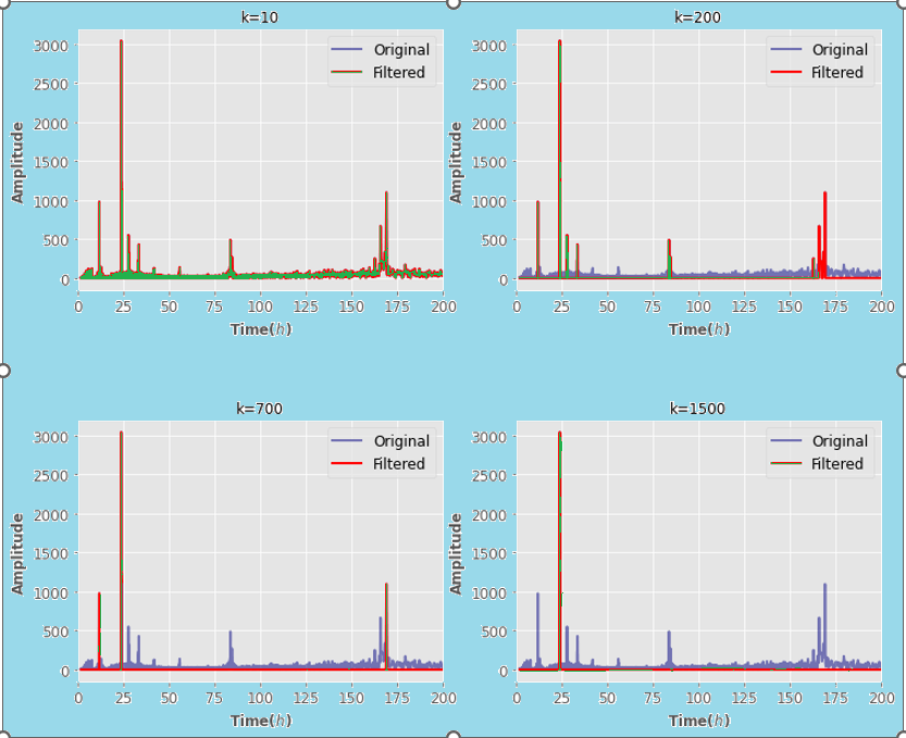
Step 7: Noise Filterings (Wavelet Transform) We can do commotion sifting utilizing the Wavelet Change too. There are multiple levels of filtering in this instance. The principal levels will channel the unadulterated clamor. However, they will be moderate. While there will be less noise as you go deeper, you will also lose some of the signal's characteristics (the residuals will be similar to the original signal). Source code: Step 8: Amplitude Extraction I just came up with an up-and-down signal for this part. Imagine that we only want to extract its envelope, also known as the amplitude. Use the scipy Hilbert Transform to determine the absolute value. Source code: Super simple and extremely useful for a data scientist who works with signals daily. 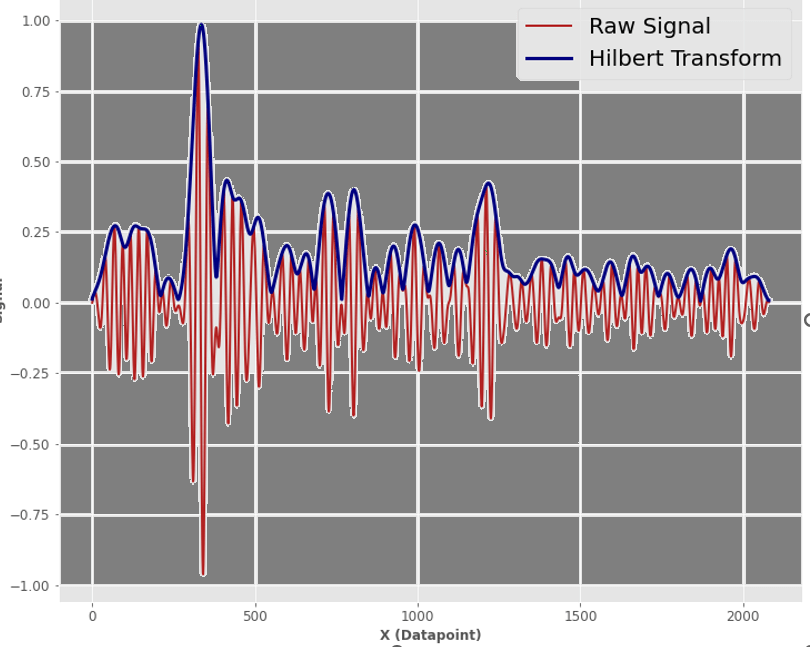
Consolidated code: Output: 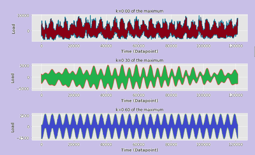
ConclusionsIf you enjoyed the article and wish to learn more about machine learning or have a question for me, you can: It will inform you of upcoming stories and allow you to text me with any questions or corrections. Join as a suggested member to read all the articles we (and dozens of other top authors in statistical machine learning) have to say on the newest technology without being limited to the "max number of publications for the month".
Next TopicScatter() plot pandas in Python
|
 For Videos Join Our Youtube Channel: Join Now
Feedback
- Send your Feedback to [email protected]
Help Others, Please Share


