Water Quality Analysis

One of everyone's basic necessities is access to clean water for drinking. Legally speaking, having access to clean water for consumption is a fundamental human right. Water quality is influenced by a variety of factors and is one of the main topics of machine learning research. So this tutorial is for you if you want to understand how to analyse water quality using machine learning. We'll lead you through a Python machine learning examination of water quality in this tutorial.

Introduction: Water Quality Analysis

Analysing water quality is one of the key topics of machine learning research. In order to train a machine learning model that can determine if a certain water sample is safe or unsafe for eating, we must first understand all the parameters that impact water potability. This process is also known as water potability analysis.

We'll be utilising a Kaggle dataset that includes information on all of the key elements that have an impact on the potability of water for the water quality analysis challenge. Before building a model using machine learning to predict whether the water specimen is acceptable or unsafe for eating, we must first quickly examine each characteristic of this dataset because all of the elements that determine water quality are crucial.

About dataset

Content

The water_potability dataset contains different types of water quality metrics.

1. The pH value is a crucial factor in determining how acidic or basic water is. Additionally, it shows if the water is acidic or alkaline. The highest pH allowed range, according to WHO, is between 6.5 and 8.5. The present investigation's ranges fell between 6.52 to 6.83, which is within WHO criteria.
2. Hardness: Salts of calcium and magnesium are the major contributors to hardness. These salts are released by the geologic formations that water passes through. How long water is exposed to a hardness-producing substance influences how hard the water is while it is in its raw state. The ability of water to form soap due to calcium and magnesium precipitation was the original definition of hardness.
3. Solids: A vast variety of inorganic and certain organic minerals or salts, such as calcium, potassium, sodium, bicarbonates, chloride compounds, magnesium, sulphates, etc., may be dissolved by water. These minerals gave the water an undesirable taste and diminished colour. This is a crucial variable while using water. Water with a high TDS rating is one that has a high mineral content. The recommended TDS level for drinking purposes is 500 mg/l, with a maximum limit of 1000 mg/l.
4. Chloramines: The two main disinfectants utilised in water supply systems in cities are chlorine and chloramine. When methane is added to bleach to purify drinking water, chloramines are most frequently generated. In drinking water, chlorine concentrations up to 4 milli-grammes per litre are regarded as safe.
5. Sulphate: Sulphates are organic compounds that are naturally present in rocks, soil, and minerals. They can be found in the surrounding air, groundwater, vegetation, and food. Sulphate is mostly used in the chemical industry for commercial purposes. In saltwater, there are around 2,700 milli-grammes of sulphate per lite. The majority of freshwater sources have concentrations between 3 and 30 mg/L, while certain regions have substantially greater levels.
6. Conductivity: Water that is clean is an excellent insulator and poor conductor of electrical current. The electrical resistance of water is improved by an increase in ion concentration. The electrical conductivity of water is typically determined by the amount of dissolved particles present. The ability of a solution to conduct electricity is determined by its ionic process, which is measured by electrical conductivity. According to WHO guidelines, the EC value shouldn't be more than 400 S/cm.
7. Organic_carbon: Both manufactured and naturally occurring organic matter ( NOM ) contribute to the total organic carbon in source waters. The total amount of carbon ( TOC ) in organic substances in pure water is a measurement of this. US EPA estimates that treated drinking water has 2 mg/L of TOC and that source water, which is used for treatment, contains 4 mg/Lit.
8. Trihalomethanes ( THMs ): THMs are substances that may be present in chlorine-treated water. The amount of organic matter in the water, the quantity of chlorine needed to treat the water-based, and the temperature of the treated water all affect the levels of THMs in drinking water. THM concentrations up to 80 ppm are regarded as safe for drinking water.
9. Turbidity: The amount of solid stuff in the water's suspended state determines how turbid it is. The test is used to determine the quality of waste released with regard to colloidal particles and measures the light-emitting capabilities of water. The Wondo Genet Campus's mean turbidity value ( 0.98 NTU ) is less than the WHO-recommended threshold of 5.00 NTU.
10. Potability: A score between 0 and 1 that indicates whether water is suitable for human consumption.

Python Water Quality Analysis

We'll begin the work of analysing the water quality by importing the dataset and the required Python libraries:

Source Code Snippet:

Output:

Before continuing, let's eliminate all the rows that have null values since I can see them in the dataset's initial preview:

Source Code Snippet:

Output:

ph                 0
Hardness           0
Solids             0
Chloramines        0
Sulfate            0
Conductivity       0
Organic_carbon     0
Trihalomethanes    0
Turbidity          0
Potability         0
dtype: int64

Input:

Output:

Input:

Output:

RangeIndex: 3276 entries, 0 to 3275
Data columns ( total 10 columns ):
 0   Column           Non-Null Count  Dtype  
- - - - - - - - - - - - - - - - - - - - - - - - - - - - - - -- - - - - - - - - - - - - - - - - - - - - - - - - - - - - - - 
 0   ph               2785 non-null   float64
 1   Hardness         3276 non-null   float64
 2   Solids           3276 non-null   float64
 3   Chloramines      3276 non-null   float64
 4   Sulfate          2495 non-null   float64
 5   Conductivity     3276 non-null   float64
 6   Organic_carbon   3276 non-null   float64
 7   Trihalomethanes  3114 non-null   float64
 8   Turbidity        3276 non-null   float64
 9   Potability       3276 non-null   int64  
dtypes: float64( 9 ), int64( 1 )
memory usage: 256.1 KB

Input:

Output:

Hardness           3276
Solids             3276
Chloramines        3276
Sulfate            2495
Conductivity       3276
Organic_carbon     3276
Trihalomethanes    3114
Turbidity          3276
Potability            2
dtype: int64

Input:

Output:

Sum values
- - - - - - - - - - - - - - - - - - - - - - - - - - - - - - - - -            
Hardness             0
Solids               0
Chloramines          0
Sulfate            781
Conductivity         0
Organic_carbon       0
Trihalomethanes    162
Turbidity            0
Potability           0
dtype: int64

Input:

Output:

ph                 float64
Hardness           float64
Solids             float64
Chloramines        float64
Sulfate            float64
Conductivity       float64
Organic_carbon     float64
Trihalomethanes    float64
Turbidity          float64
Potability           int64
dtype: object

Since this dataset's Potability column comprises values 0 and 1, which represent whether the water in the system is fit for eating or not ( 0 ), it is this column that we must predict. Check out the breakdown of 0 and 1 in the column for potability now:

Source Code Snippet:

Output:

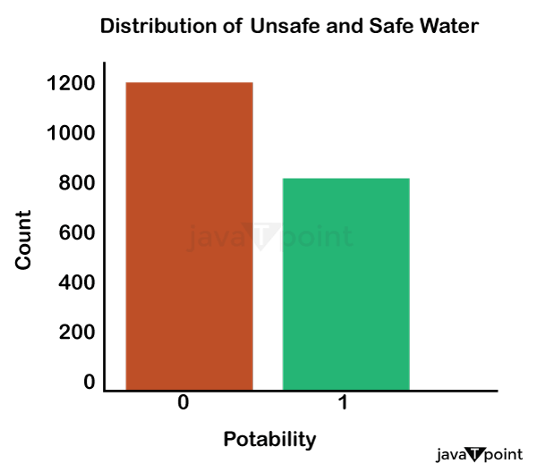
You should be aware that this dataset has an imbalance because there are more samples of 0s than 1s.

We can overlook no elements that have an impact on water quality, as was already said, therefore let's look at each column individually. Let's begin by examining the ph column:

Source Code Snippet:

Output:

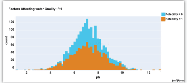
The ph column shows the water's ph value, which is crucial for determining the water's acid-base balance. Drinking water should have a pH level of 6.5 to 8.5. Let's examine the dataset's second element impacting water quality now:

Source Code Snippet:

Output:

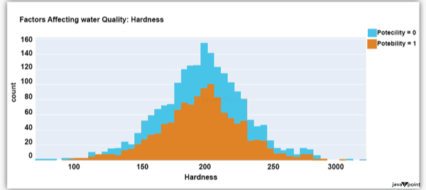
The distribution of fluid hardness in the dataset is depicted in the image above. Water's hardness often varies depending on where it comes from, however water between 120 and 200 milligrammes is drinkable. Let's now examine the following element impacting water quality:

Source Code Snippet:

Output:

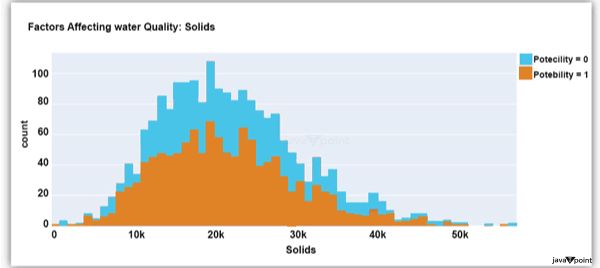
The dataset's distribution of all of the dissolved solids in water is shown in the figure above. Dissolved solids are any organic or inorganic minerals found in water. Highly mineralized water has a very high dissolved solids content. Let's now examine the next element impacting water quality:

Source Code Snippet:

Output:

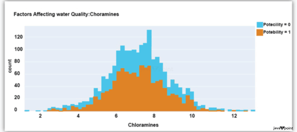
The dataset's distribution of chlorine dioxide in water is shown in the image above. In public water systems, disinfectants like chlorine and chloramine are employed. Let's now examine the following element impacting water quality:

Source Code Snippet:

Output:

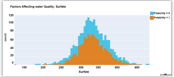
The dataset's distribution of sulphate in water is seen in the figure above. They are elements that occur naturally in minerals, soil, and rocks. Drinkable water is defined as having less than 500 mg of sulphate. Next, let's examine another element:

Source Code Snippet:

Output:

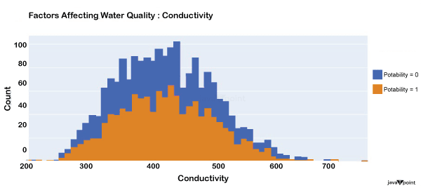
The distribution of a fluid's conductivity in the dataset is shown in the image above. The most pure type of water is not an effective conductor of electricity, although water is an excellent conductor of electricity in general. Drinkable water has an electrical resistance of less than 500. Next, let's examine another element:

Source Code Snippet:

Output:

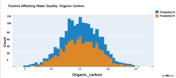
The dataset's distribution of carbon compounds in water is shown in the image above. Decomposition of organic substances from both natural and artificial sources yields organic carbon. Drinkable water is defined as having fewer than 25 milligrammes of organic carbon. Let's now examine the following element that has an impact on drinking water quality:

Source Code Snippet:

Output:

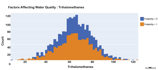
The distribution of trihalomethanes, or THMs, in water is shown in the image above. Water that has been chlorinated contains compounds called THMs. Drinkable water is defined as having fewer than 80 milligrammes of THMs. Let's now examine the following variable in the dataset that influences the quality of drinking water:

Source Code Snippet:

Output:

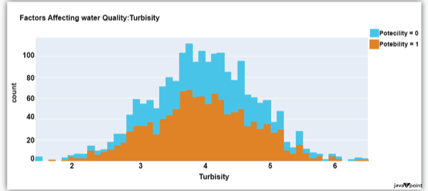
The distribution of turbidity in water is seen in the above graph. The quantity of suspended particles affects the turbidity of water. Drinkable water is defined as having less than 5 milli-grammes of turbidity.

Python-based Water Quality Prediction Model

All the elements that influence water quality were discussed in the section above. The following step is to use Python to build a model based on machine learning for the purpose of analysing water quality. I'll be utilising the Python PyCaret package for this purpose. If you've never used this package of libraries before, using the pip command, you can quickly install it on your system:

• pycaret installation

Let's look at the association between all the characteristics and the dataset's Potability column before building a machine learning model:

Source Code Snippet:

Output:

ph                 1.000000
Hardness           0.108948
Organic_carbon     0.028375
Trihalomethanes    0.018278
Potability         0.014530
Conductivity       0.014128
Sulfate            0.010524
Chloramines       -0.024768
Turbidity         -0.035849
Solids            -0.087615
Name: ph, dtype: float64

The PyCaret Python module is now used to determine which machine learning method is appropriate for this dataset:

Source Code Snippet:

Output:

The aforementioned result indicates that training a model based on machine learning for the purpose of analysing water quality is best accomplished using the random forecast classifying technique. Therefore, let's train the algorithm and assess its forecasts:

Source Code Snippet:

Output:

The findings shown above appear to be good. I hope you enjoyed my Python-based machine learning experiment on analysing water quality.

Summary

So this is how you may evaluate the water's quality and train a machine learning model to distinguish between water that is safe to drink and water that is not. One of everyone's basic necessities is access to clean water for drinking. Legally speaking, having access to clean water for consumption is a fundamental human right. Water quality is influenced by a variety of factors and is one of the main topics of machine learning research. I hope you enjoyed reading this tutorial on Python-based machine learning for water quality analysis. Please feel free to leave your insightful remarks via mail.